Setup
Let’s load the {ggplot2} library and create two basic ggplots, stored as g1 (scatter plot) and g2 (box-and-whisker plot) that can be used later.
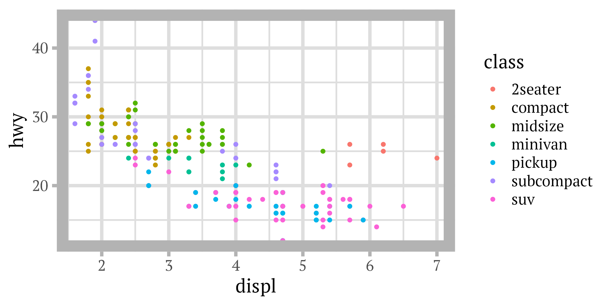
g1 <- ggplot(mpg, aes(x = displ, y = hwy)) +
  geom_point(aes(color = class))

g1
g2 <- ggplot(mpg, aes(x = class, y = hwy)) +
geom_boxplot()
g2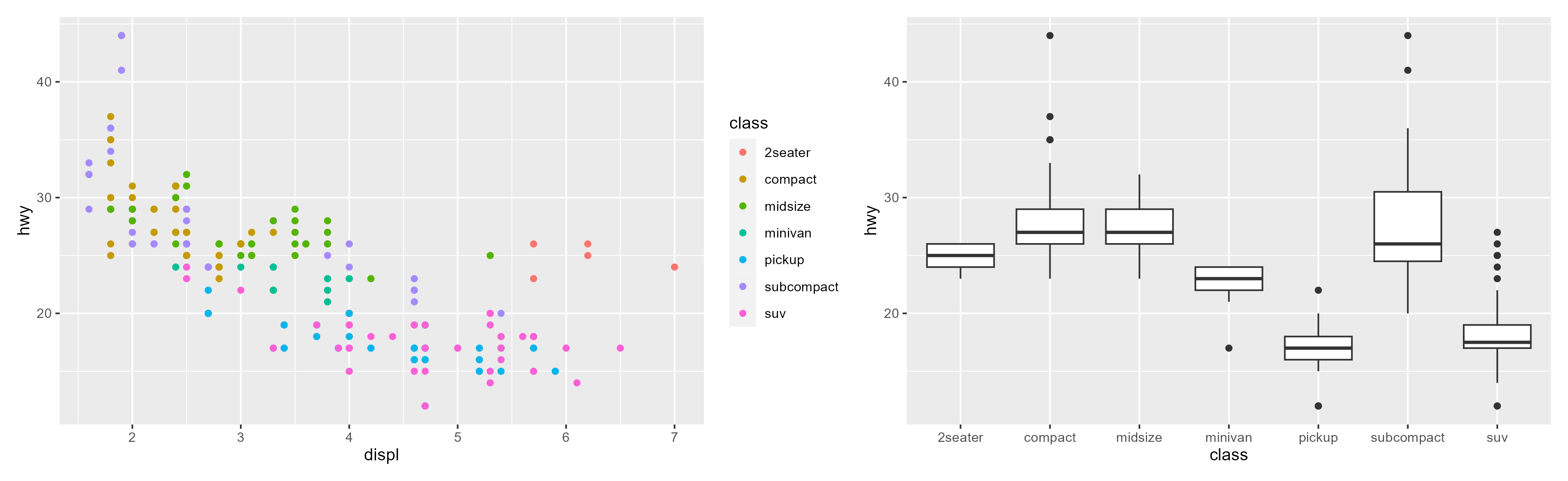
Theming
The resulting plots use the default gray theme: theme_gray() or theme_grey().
We can change the default theme by adding a complete theme, starting with theme_*(), and/or customizing single elements of the default theme via theme():
g1 +
  ## apply light complete theme
  theme_light() +
  ## remove minor grid + modify typeface
  theme(panel.grid.minor = element_blank(),
        text = element_text(family = "PT Sans"))
g2 +
theme_light() +
theme(panel.grid.minor = element_blank(),
text = element_text(family = "PT Sans"))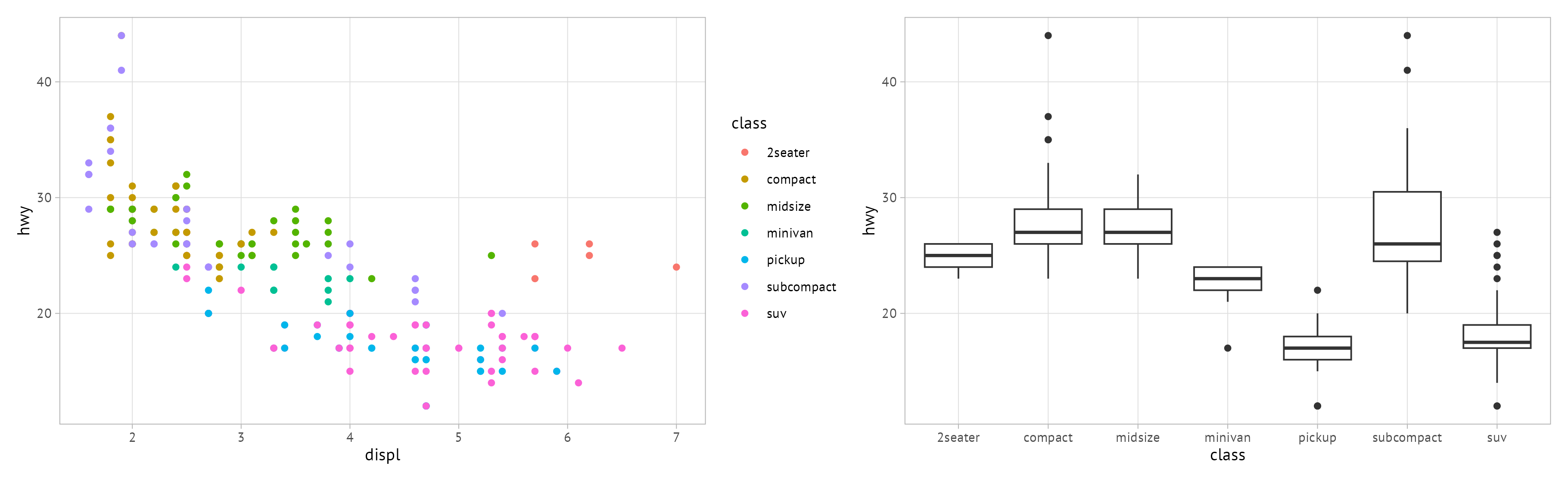
This procedure involves a lot of copy-and-paste’ing, which makes it a tedious procedure especially in case you decide to make some general styling changes at a later point. It is also prone to mistakes as you might forget to set specific adjustments for single plots.
Check also our D6 corporate theme which is part of our {d6} R package and the respective blog post! The theme comes with a larger base size and several additional arguments to simplify customization with regard to typefaces, grid lines, margins and more.
Set Themes Globally
Instead of repeating the same code to change the appearance of your plots, it is more efficient and beneficial to overwrite the default global theme:
After setting the new theme, all plots created within the same environment are styled accordingly:
g1g2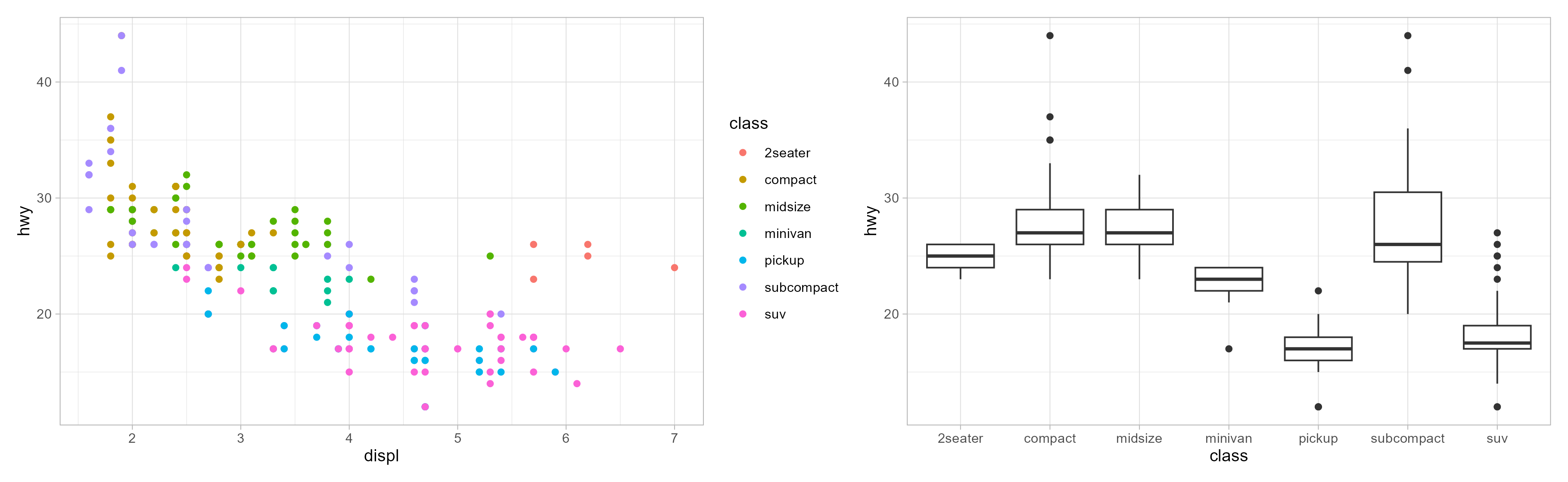
Adjust Theme Base Settings
Complete themes allow for some general modifications, no matter if added locally to your plot or if set globally. The setting include the typeface used for all text elements (base_family), the general base size (base_size) as well as dedicated relative sizes for line elements (base_line_size) and rect elements (base_rect_size).
g1 +
  theme_light(
    base_family = "PT Serif", ## default: depends on OS
    base_size = 18,           ## default: 11
    base_line_size = 3,       ## default: base_size/22 -> 0.5
    base_rect_size = 10       ## default: base_size/22 -> 0.5
  )
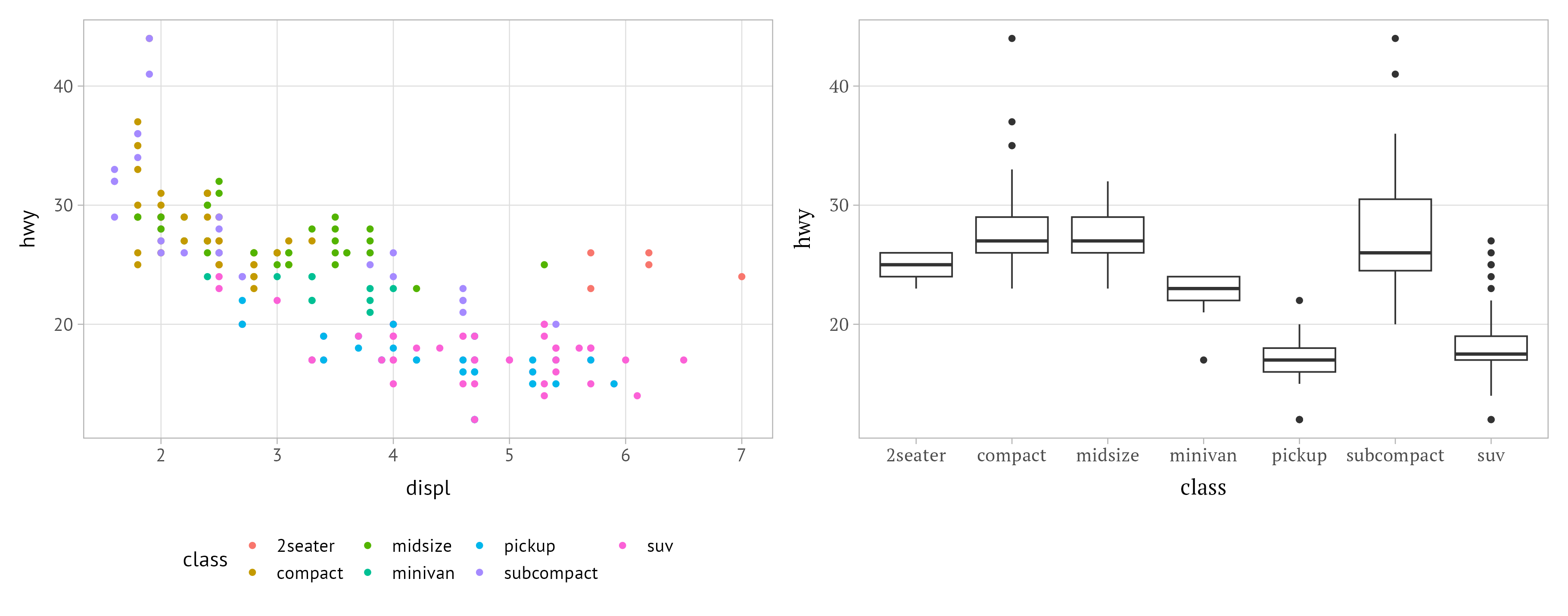
Knowing of this feature, we can already adjust the general size (which tends to be too small by default) as well as the typeface of our custom global theme:
theme_set(theme_light(base_size = 15, base_family = "PT Sans")) … which is then used for all following plots:
g1g2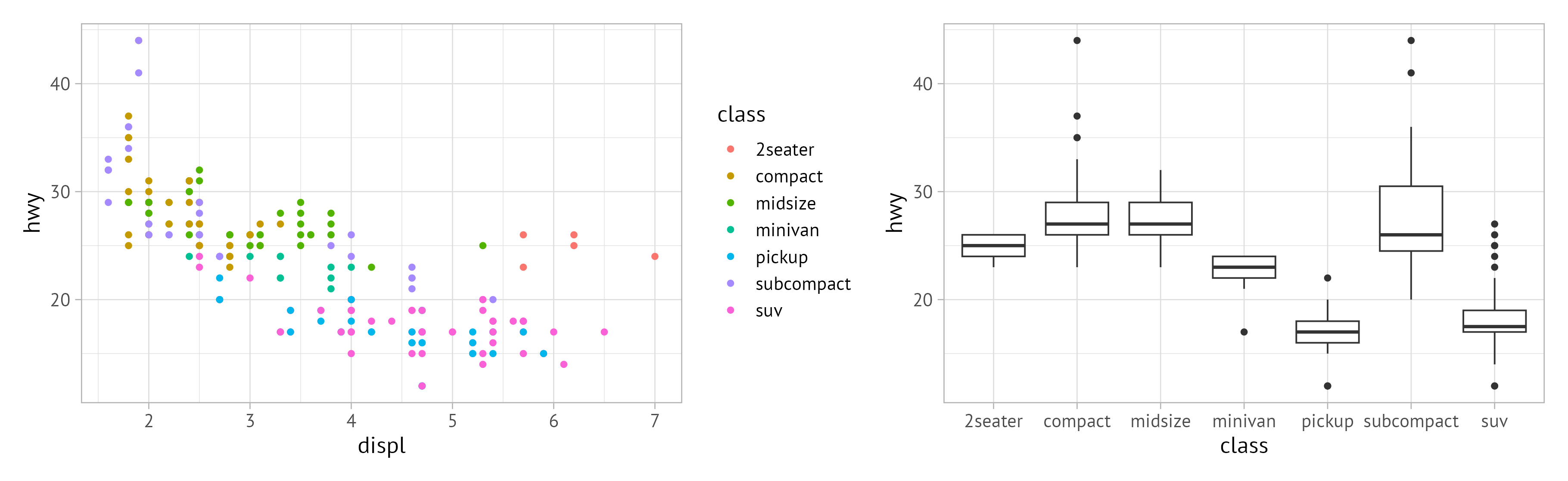
Update Theme Elements
Complete themes are great but in most circumstances we likely want to adjust a few things. Usually, you do that by adding the theme() function to your ggplot (as shown in the beginning). However, similarly to theme_set() we can apply the modifications globally:
theme_update(
  panel.grid.minor = element_blank(),
  axis.title = element_text(face = "bold"),
  legend.title = element_text(face = "bold")
)g1g2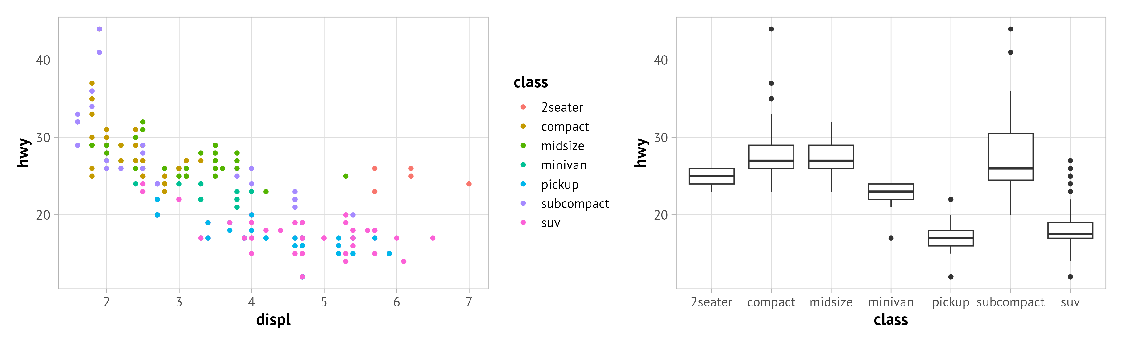
Custom Local Modifications
Of course, you can still either overwrite the global theme as before or modify specific elements for a single plot if needed:
g1 +
  ## new complete theme
  theme_classic(base_family = "PT Serif", base_size = 15) +
  ## add grid lines
  theme(panel.grid.major = element_line(color = "grey90"))
g2 +
## remove vertical grid lines + overwrite axis title styling
theme(panel.grid.major.x = element_blank(),
axis.title = element_text(color = "red", face = "italic")) 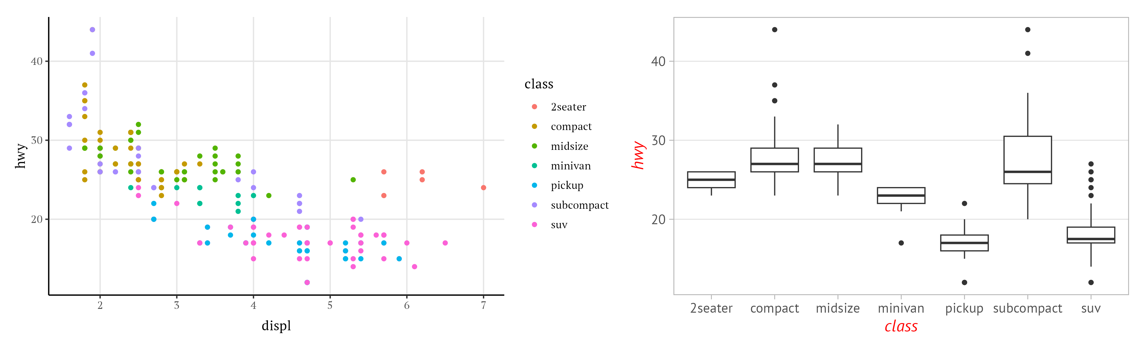
Summary
Setting and updating ggplot themes globally is efficient and avoids potential mistakes.
As a workflow routine, add a chunk that loads {ggplot2} and afterwards sets and updates your theme at the beginning of a script rather than adding the same code to each plot individually.
Multi-Panel Figures
We often use multi-panel visualizations, i.e. several plots layed out in a single graphic. Instead of combining single figures manually, we make use of a coding-first approach.
There are many packages to combine ggplots such as {gridExtra}, {cowplot}, and {ggarrange}. The most recent, and IMHO the best in terms of functionality and simplicity, is the {patchwok} package by Thomas Lin Pedersen. For simple multi-panel graphics, mathematical operators can be used – easy to use and remember.
g1 + g2
g1 / g2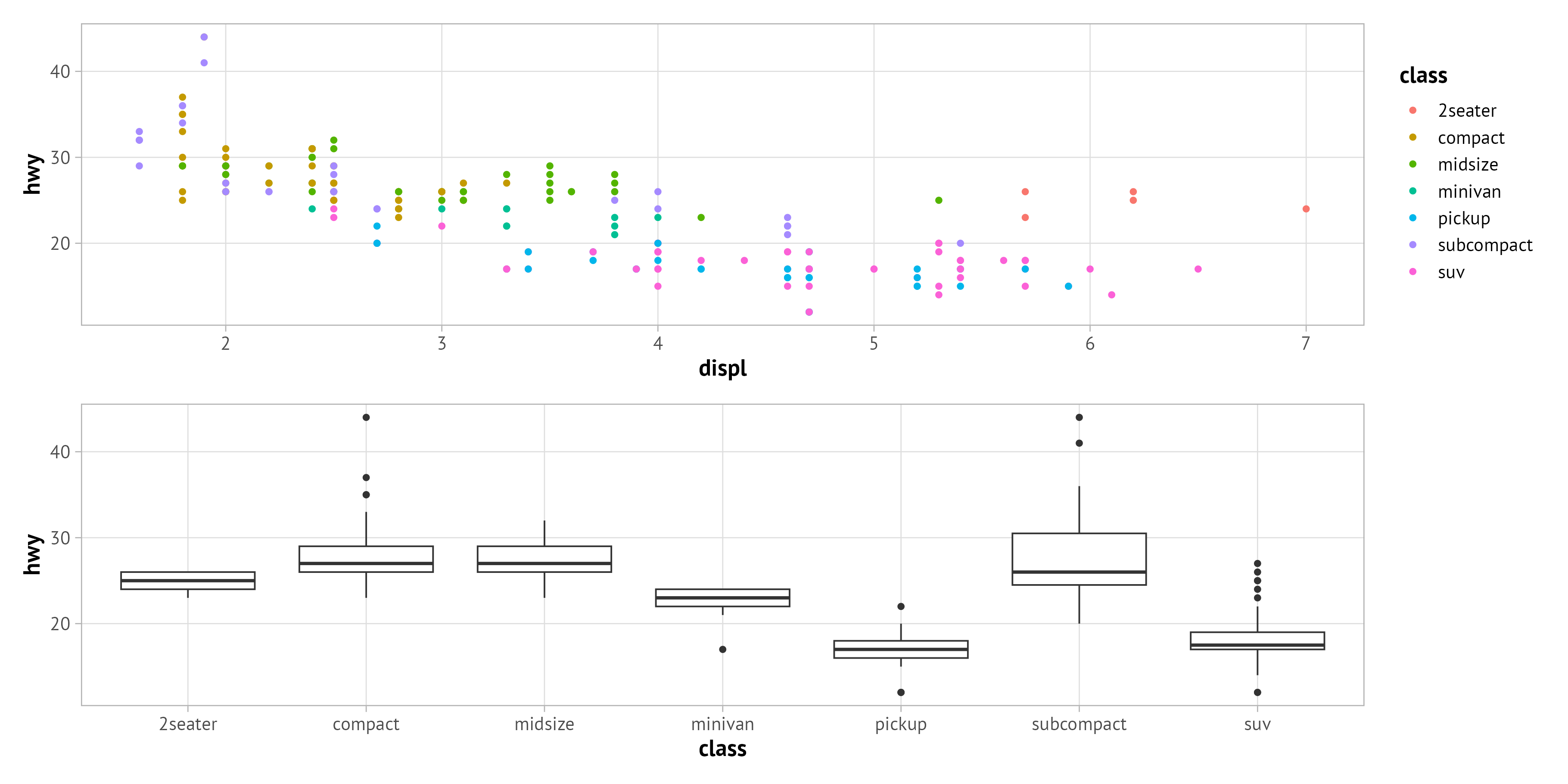
Adjust Layout
By default, both plots take the same space. In case you want to adjust how the plots are laid out, use plot_layout() in combination with either widths or heights. These arguments take a vector with the relative width or height for each plot, respectively.
g1 + g2 +
  plot_layout(widths = c(.5, 1))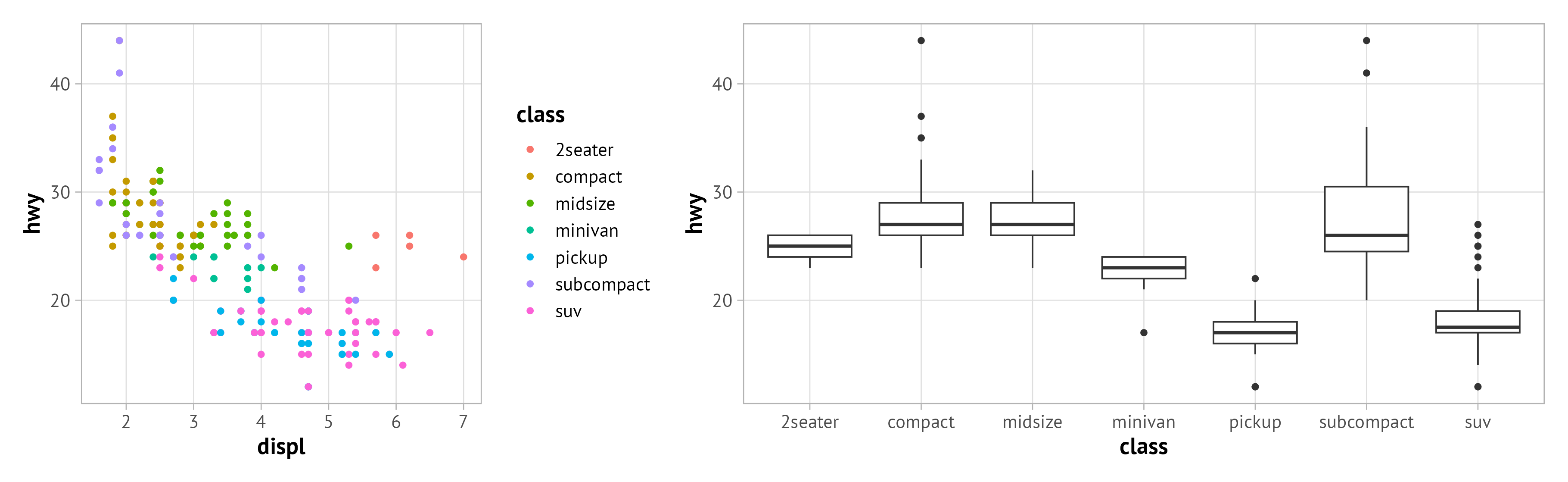
Add White Space
{patchwok} comes with a placeholder to add empty space between plots. Once can add a plot_spacer() similar to a regular plot:
g1 + plot_spacer() + g2 +
plot_layout(widths = c(.5, .1, 1))![]()
Nested Layouts
Also more complex layouts can be created:
(g1 + g3 + g4) / (g2 + g5)
Code to create g3, g4, and g5
g3 <- ggplot(mpg, aes(x = cyl, y = hwy)) +
  geom_point(aes(color = class))

g4 <- ggplot(mpg, aes(x = cty, y = hwy)) +
  geom_point(aes(color = class))

g5 <- ggplot(mpg, aes(x = class, y = hwy)) +
  stat_summary(fun.data = "mean_sdl", fun.args = list(mult = 1))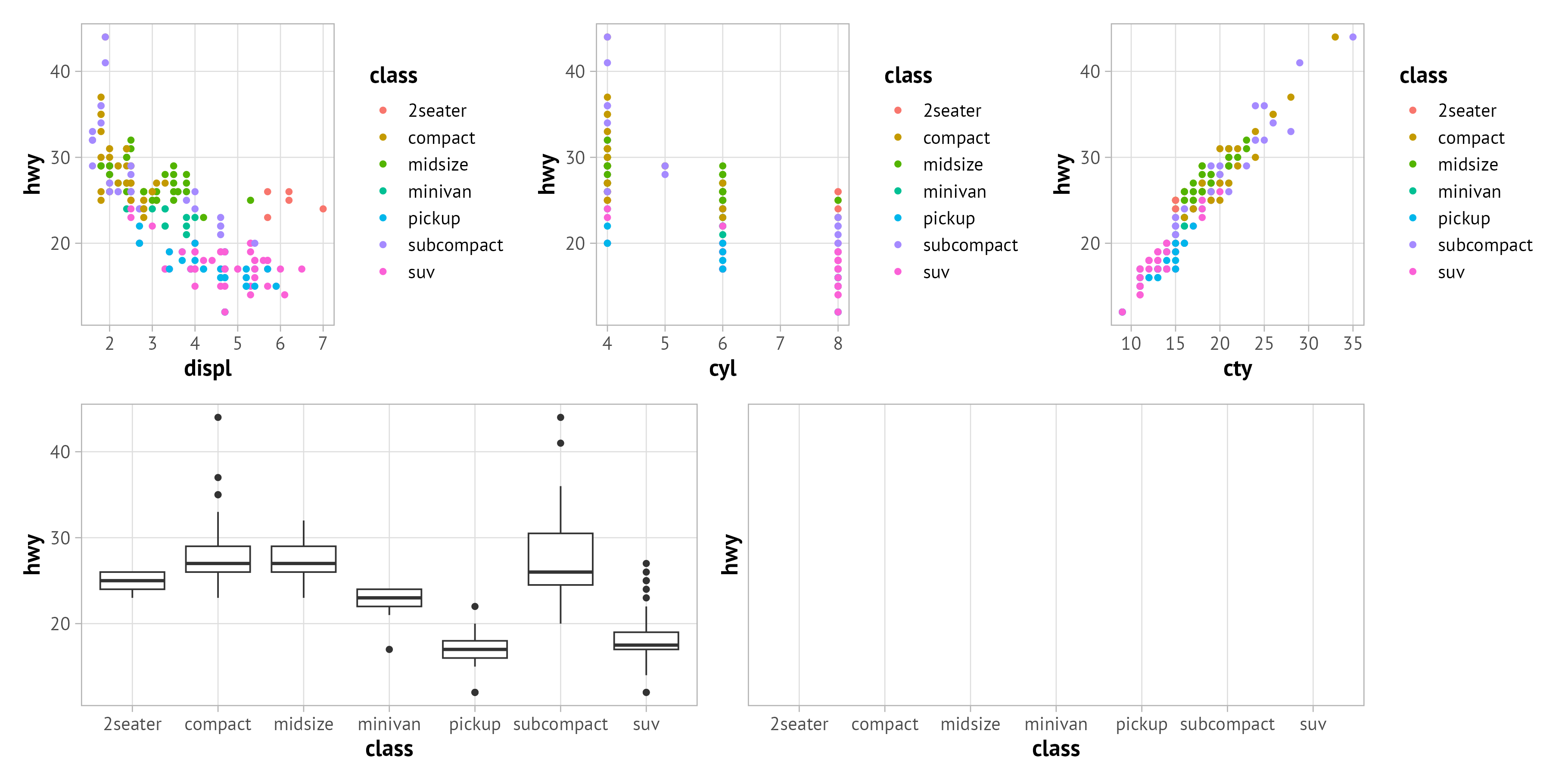
Alternatively, you can also create a design layout to have full control:
layout <-
  "
  ABBCCC#
  DDDD#EE
  "

g1 + g3 + g4 + g2 + g5 +
  plot_layout(design = layout)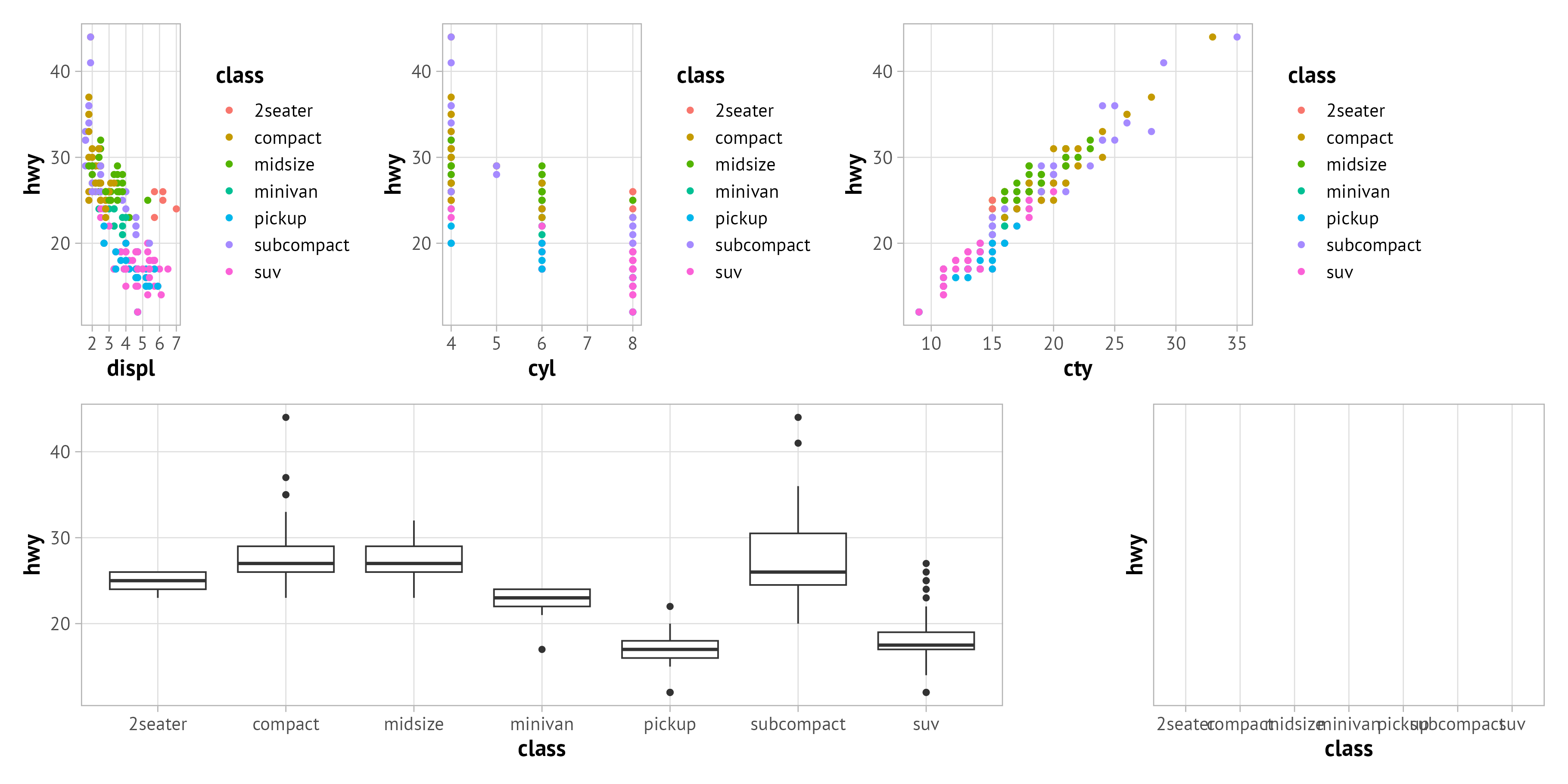
The letters refer to the single plots (in the order you combine them later) and a hash # indicates empty space, similar to plot_spacer().
Merge Legends
Displaying the legend three times makes no sense. {patchwork} offers the utility to “collect your guides” inside the plot_layout() function:
(g1 + g3 + g4) / (g2 + g5) +
  plot_layout(guides = "collect")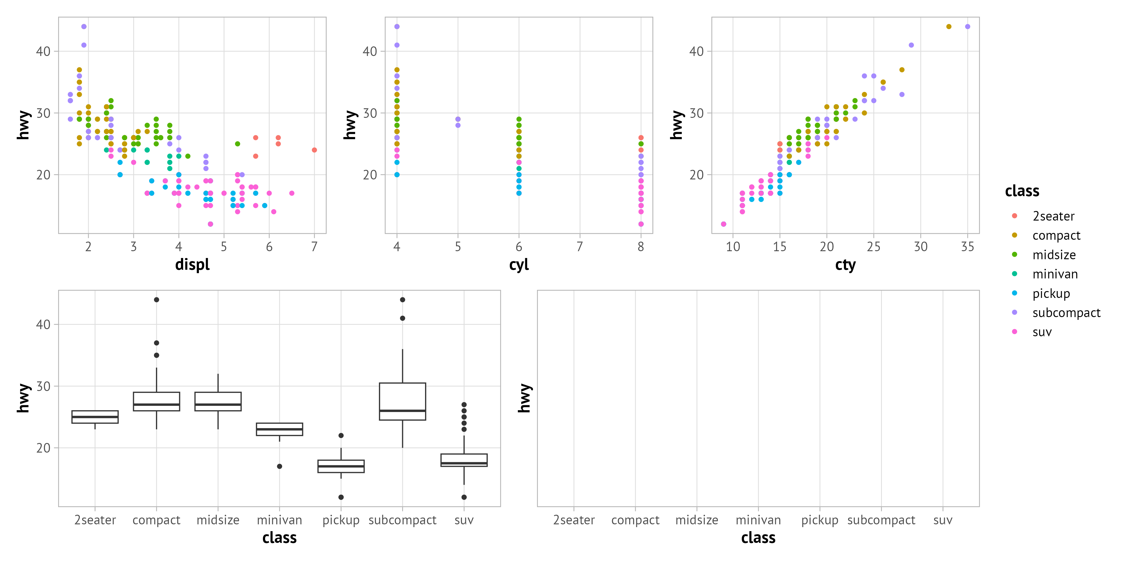
Now we may want to move it to the top so it is shown next to the relevant colored scatter plots, not in the middle. We can adjust the theme for all plots inside another {patchwork} function called plot_annotation()—or by updating your global theme 😉
((g1 + g3 + g4) / (g2 + g5)) +
  plot_layout(guides = "collect") +
  plot_annotation(theme = theme(legend.justification = "top"))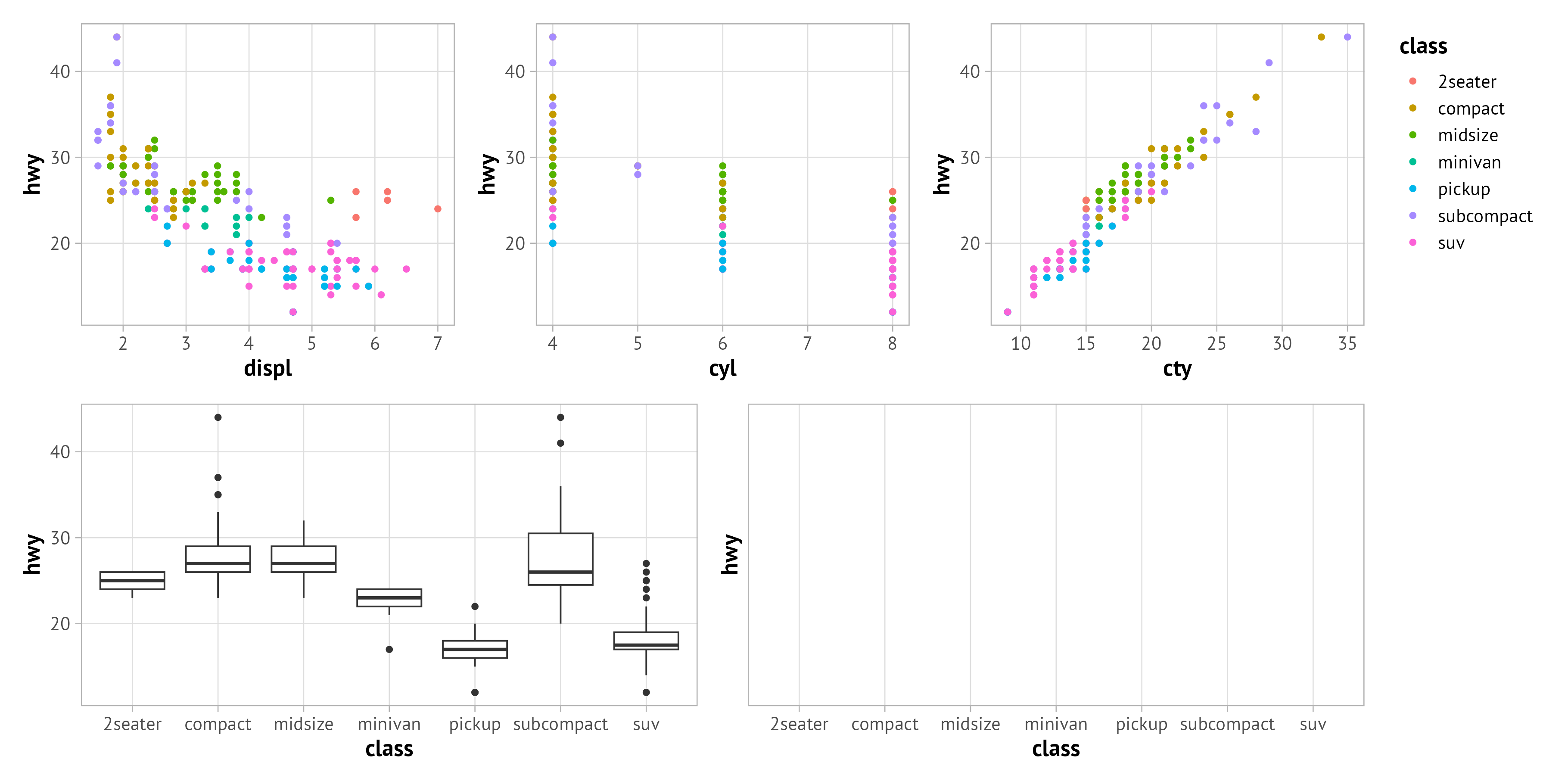
Automate Plot Tags
When preparing such multi-panel figures for publications, we usually want to add tags to be able to refer to subplots in the figure caption or main text. Again, we can do this inside R instead of adding them afterwards by hand (which either takes very long or results in irregularly aligned labels).
((g1 + g3 + g4) / (g2 + g5)) +
  plot_layout(guides = "collect") +
  plot_annotation(tag_levels = "A",
                  theme = theme(legend.justification = "top"))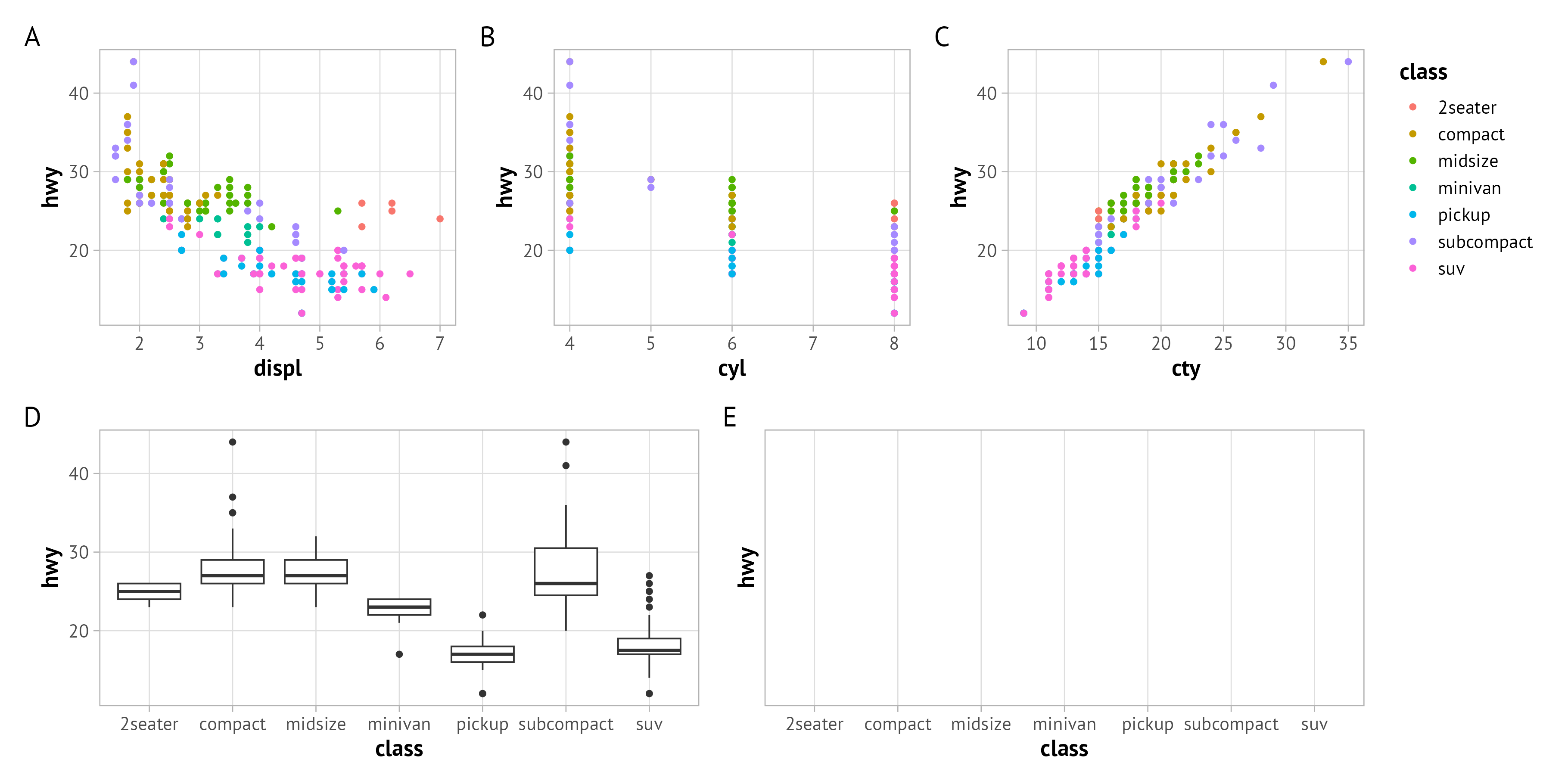
{patchwork} understands a range of numbering formats such as a for lowercase letters, 1 for numbers, or i and I for lowercase and uppercase Roman numerals, respectively. Furthermore we can style the tag by defining a pre- and/or suffix:
((g1 + g3 + g4) / (g2 + g5)) +
  plot_layout(guides = "collect") +
  plot_annotation(tag_levels = "i", tag_prefix = "(", tag_suffix = ")",
                  theme = theme(legend.justification = "top"))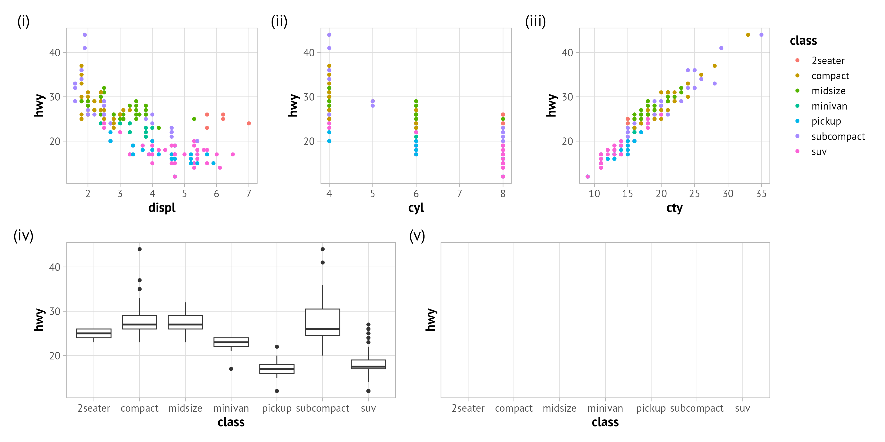
Inset Plots
Similar to other arrangement packages, we can use {patchwork} also to add inset plots. Inside the inside_element() function, we specify the plot to draw and then the outer bounds (left, bottom, right top).
g4 + inset_element(g1 + guides(color = "none"), .5, 0, 1, .5)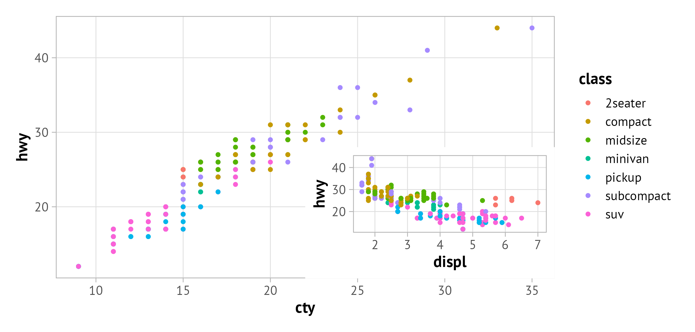
By default, the inset plot is aligned with the panel of the main plot. If you want to modify the behavior, overwrite the default input of align_to.
g4 + inset_element(g1 + guides(color = "none"), .5, 0, 1, .5, align_to = "plot")
g4 + inset_element(g1 + guides(color = "none"), .5, 0, 1, .5, align_to = "full")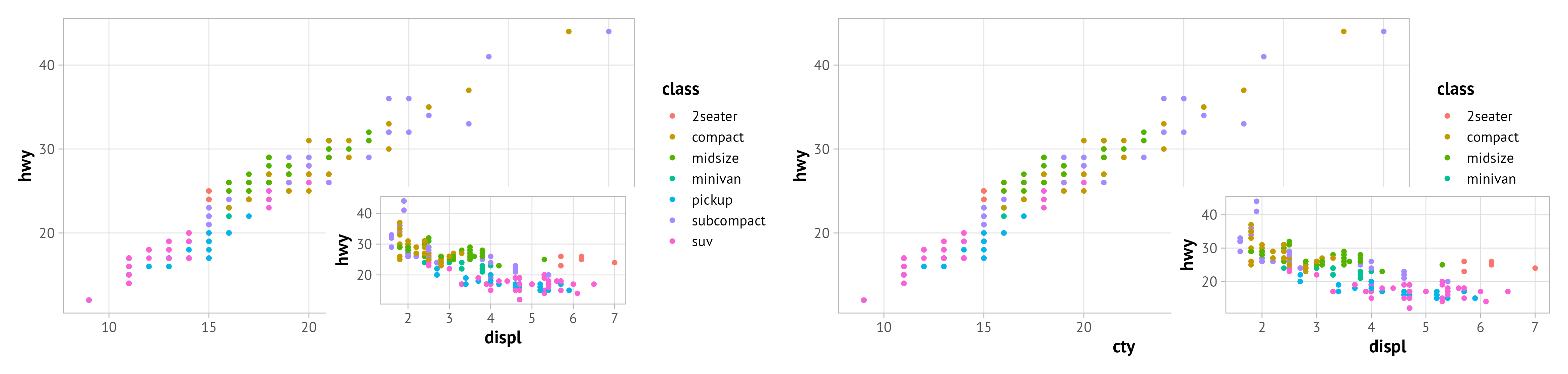
Summary
{patchwork} offers some great functionality to create basic and pretty complex layouts, add inset plots, merge repeated legends, and automate tag numbering. This makes it a powerful tool as you do not need to adjust tag labels, legends, and more for the individual ggplot.