Recently, I added a custom theme for {ggplot2} to our {d6} workflow package which makes it easy to create plots in a style that matches our lab identity used for our webpage, posters, and publications. Also, it hopefully simplifies your workflow by a ready-to-use theme with additional options that allow you to adjust the style of your ggplots.
Let us know if there is a theme feature you often modify via the theme() function! We can add it as an argument to the complete theme function.
## install (if needed) and load packages
d6::simple_load(c("ggplot2", "EcoDynIZW/d6"))
The default theme features a vertical and horizontal grid, our corporate sans font, and a transparent background. It also uses a larger default base_size of 14 pts that controls the size of text labels as well as line elements and borders (the ggplot2 default is 11 pts).
## prepare data
data <- dplyr::filter(economics_long, !variable %in% c("pop", "pce"))

## create base plot
g <-
  ggplot(data, aes(x = date, y = value01, color = variable)) +
  geom_line()

## apply corporate theme
g + d6::theme_d6()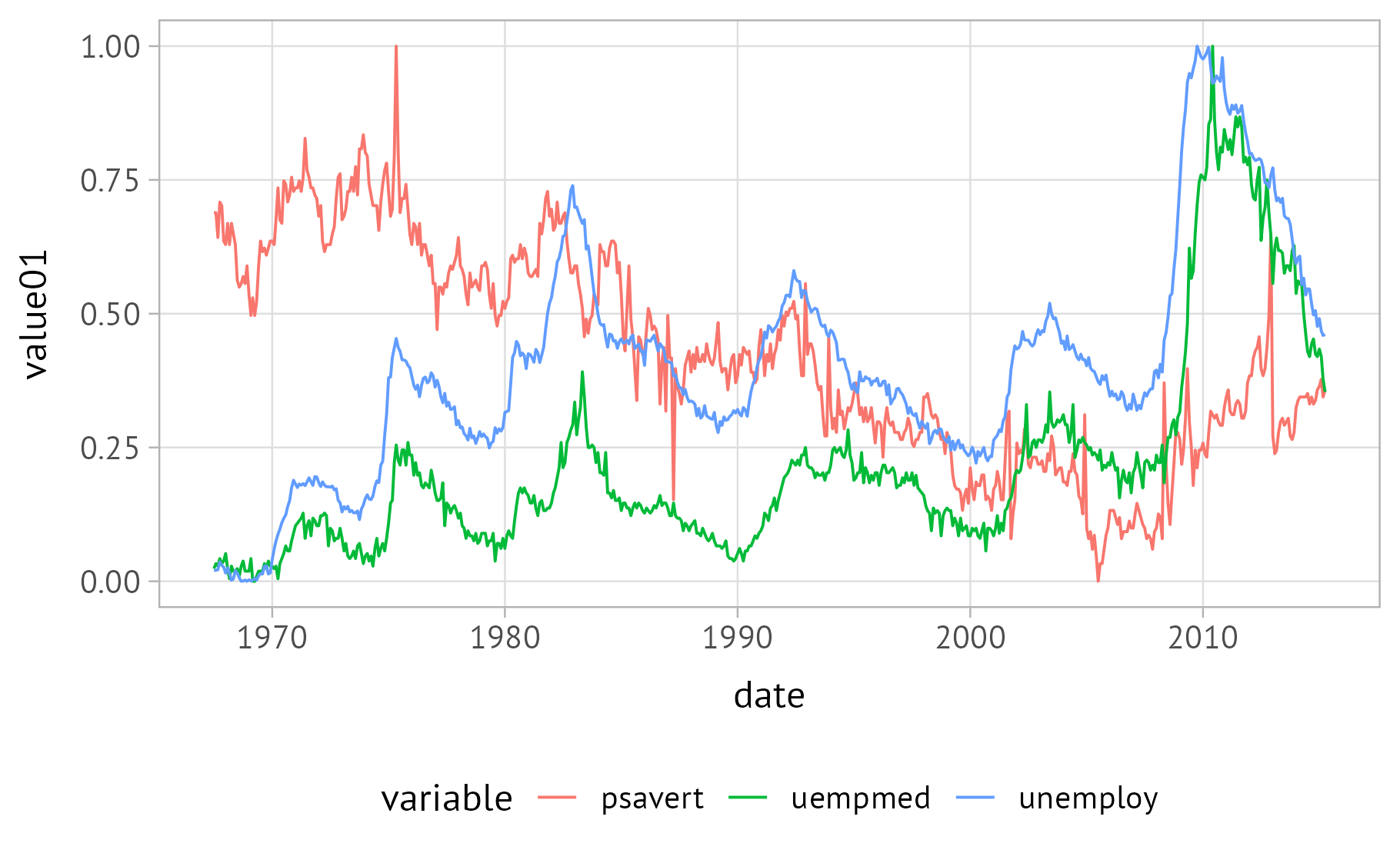
As usual with complete themes, you can overwrite the base settings, namely base_family, base_size, base_size_line, and base_size_rect:
## modify theme base setting
g + d6::theme_d6(base_size = 18, base_rect_size = 2)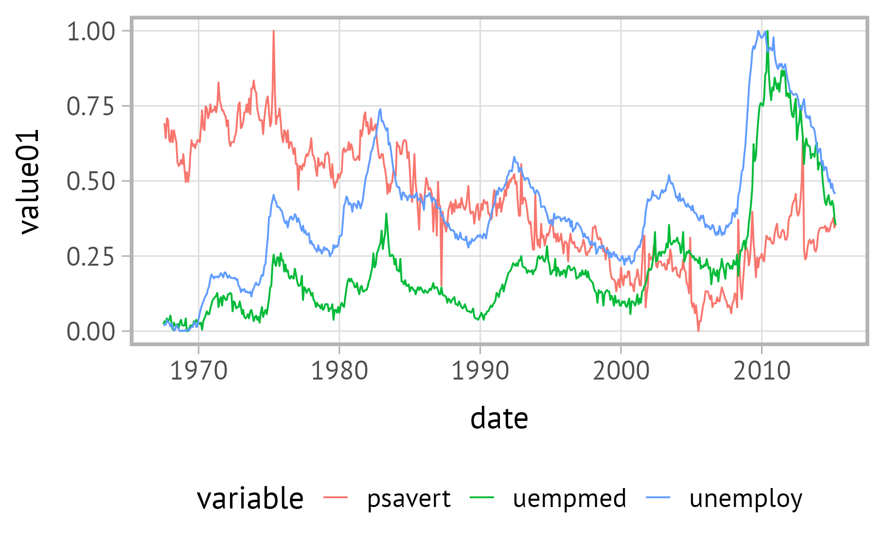
Typeface Choices
Main Typeface
The default typeface used is PT Sans. If you prefer a serif typeface, you can switch to PT Serif by setting serif = TRUE.
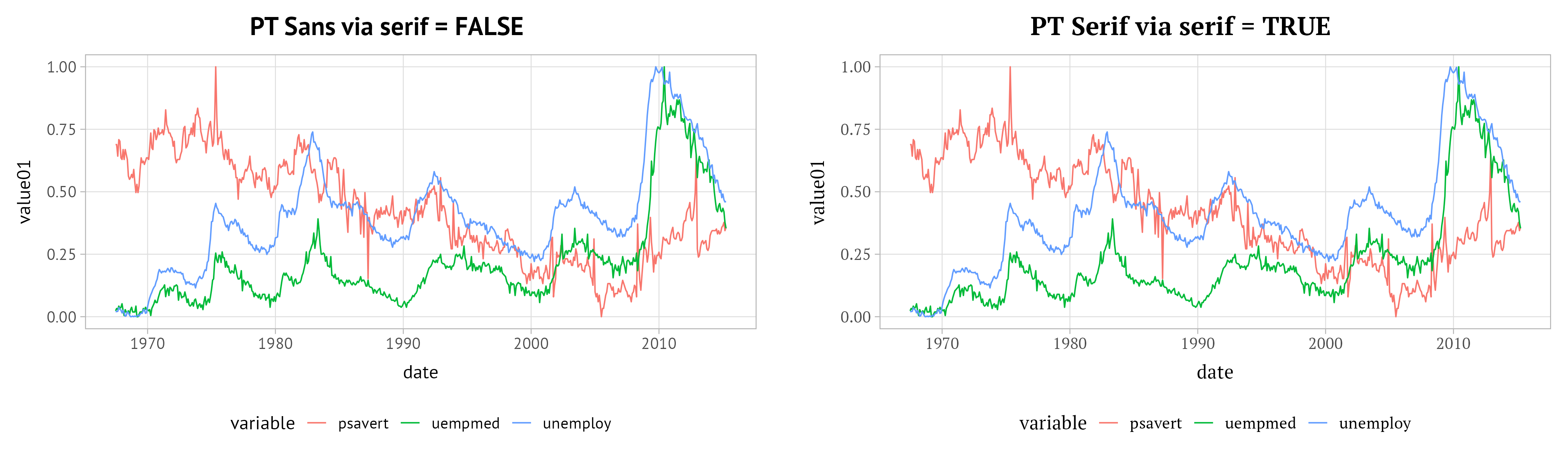
Note that the typefaces need to be installed on your machine. A warning will inform you if the relevant fonts are not installed.
Please use the {systemfonts} package to access font files as this is the most recent and best implementation to use non-default fonts in combination with {ggplot2}. Loading other font packages, especially the {showtext} package, likely cause problems.
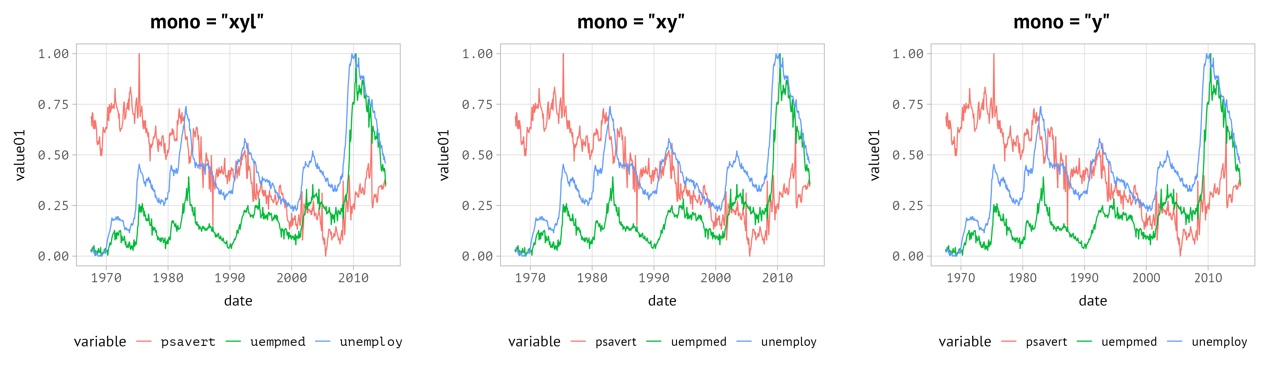
Tabular Font Option
For numeric axis labels and legends, you might want to use a tabular typeface (i.e. one where the characters all have the same width). You can set the axis and legend text individually by combining x, y, and l (uppercase letters work as well).
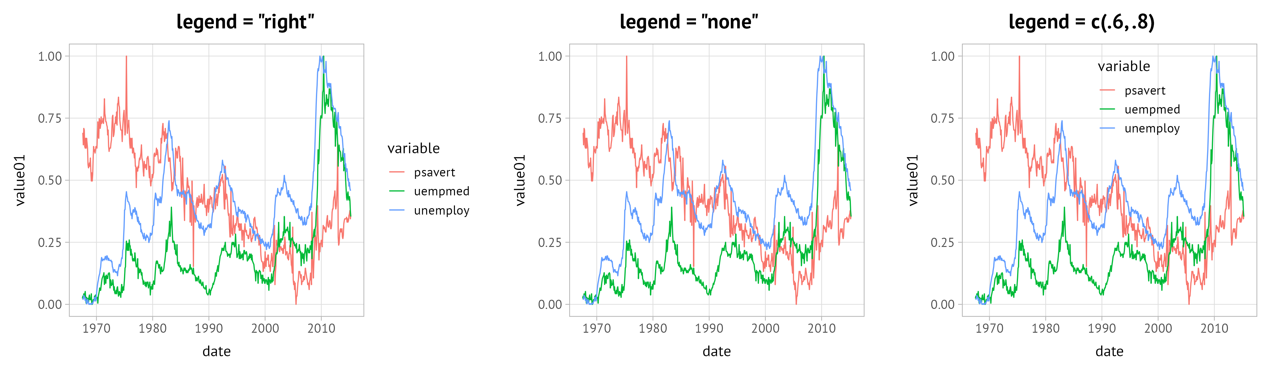
Legend Position
By default, the legend is placed at the bottom. You can easily change the position via the legend argument. This is a shortcut to theme(legend.position) and thus you can pass either strings specifying the position or a vector defining the x and y position as usual:
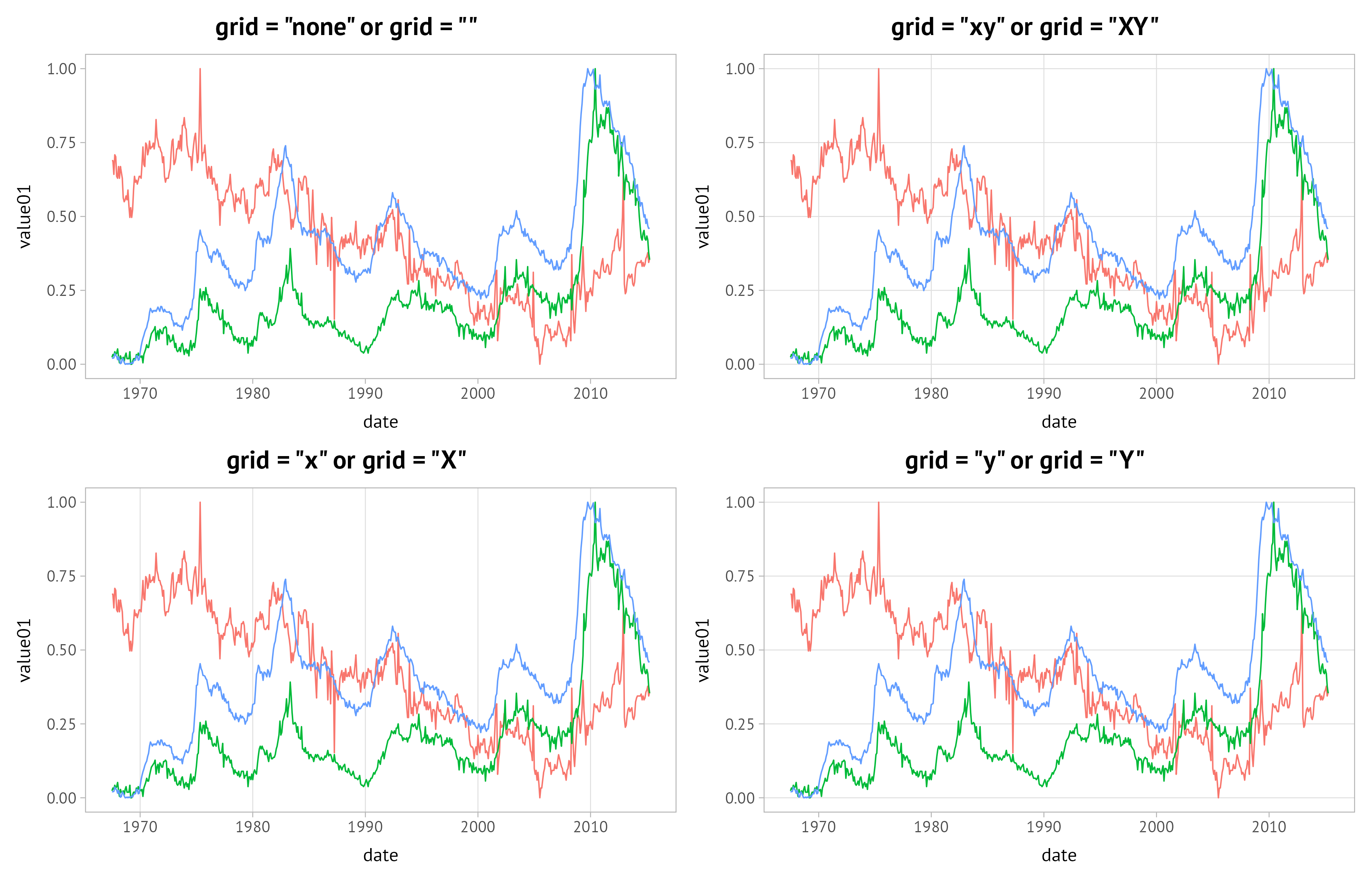
Control Grid
The default themes comes with no grid lines but you can easily add them by specifying “x” for vertical, “y” for horizontal, or “xy” for both, vertical and horizontal grid lines (uppercase letters work as well).
All theme styles do not feature minor grid lines to avoid cluttering and distractions.
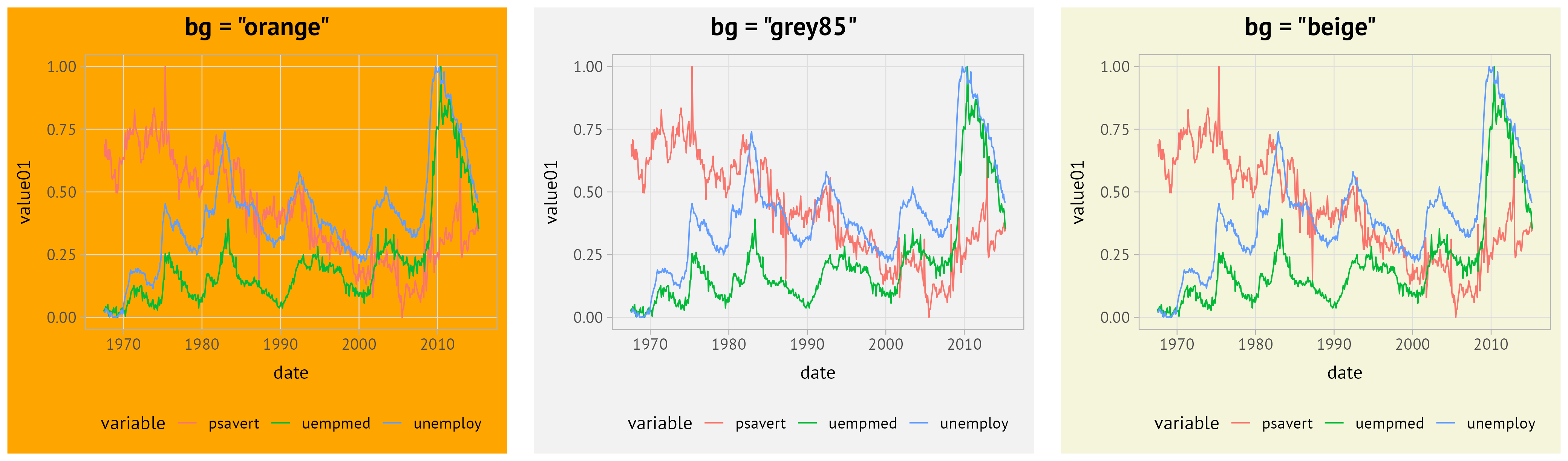
Modify Background Color
By default the background color of all boxes (plot, panel, and legends) is transparent. You can adjust the colors by passing any color name or hex code to the bg argument:
It is not possible to control individual boxes via theme_d6(). If you wish to, for example, color the background of the panel area in a different, you have to specify that via the theme() function as usual:
g + d6::theme_d6(bg = "orange") +
  theme(panel.background = element_rect(fill = "white", color = "transparent"))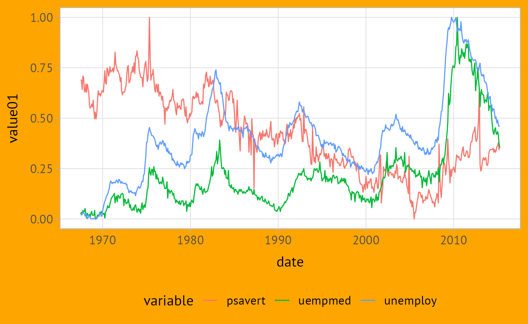
Set Plot Margin
Depending on the use case, you might want to adjust the margin around the plot. The default is related to the base_size and the same for all sides (top, right, bottom, left) specified as rep(base_size / 2, 4). You can modify the margins easily within the theme_d6().