Raster Operations

Learn how to 1) obtain a template raster from the {d6geodata} package, 2) expand the raster in different ways, 3) rasterize vector data, and 4) extract information from a raster using vector data. The methods described involve the use of packages like {terra} and {sf}, and include examples and plots to illustrate the processes. Additionally, we show how to use the {tidyterra} package for plotting raster data with {ggplot2}.

Setup

Install the {d6geodata} library and load all necessary libraries.

#remotes::install_github("EcoDynIZW/d6geodata")
library(d6geodata)
library(terra)
library(ggplot2)
library(sf)
library(patchwork)
library(dplyr)

theme_set(
  theme(axis.text.x = element_text(size = 8),
        axis.text.y = element_text(size = 8))
) 

Raster Template

First get the template raster. The origin is the extent of Berlin with the projection LAEA (EPSG:3035).

temp <- d6geodata::temp_ras(1000) # resolution is 1000m
values(temp) <- 1 # set a dummy value for visualization purposes 

temp

class       : SpatRaster 
dimensions  : 37, 46, 1  (nrow, ncol, nlyr)
resolution  : 1000, 1000  (x, y)
extent      : 4531040, 4577040, 3253790, 3290790  (xmin, xmax, ymin, ymax)
coord. ref. : +proj=laea +lat_0=52 +lon_0=10 +x_0=4321000 +y_0=3210000 +ellps=GRS80 +units=m +no_defs 
source(s)   : memory
name        : temp 
min value   :    1 
max value   :    1 

We load Berlin districts data set from our cloud to show the borders of Berlin.

berlin <- d6geodata::get_geodata(data_name = "districs_berlin_2022_poly_03035_gpkg",
                                 path_to_cloud = "E:/PopDynCloud",
                                 download_data = FALSE) %>% 
  st_union() %>% # using `st_union()` to combine geometries
  st_cast("POLYGON")

Reading layer `districs_berlin_2022_poly_03035' from data source 
  `E:\PopDynCloud\GeoData\data-raw\berlin\districs_berlin_2022_poly_03035_gpkg\districs_berlin_2022_poly_03035.gpkg' 
  using driver `GPKG'
Simple feature collection with 97 features and 6 fields
Geometry type: MULTIPOLYGON
Dimension:     XY
Bounding box:  xmin: 4531043 ymin: 3253864 xmax: 4576654 ymax: 3290795
Projected CRS: ETRS89-extended / LAEA Europe

p_berlin <- geom_sf(data = berlin, alpha = 0, color = "black", lwd = 0.7)

Now we plot the map.

p1 <- d6geodata::plot_qualitative_map(temp) # you can use this build-in plot function from the `{d6geodata}` package 
 
p1 + p_berlin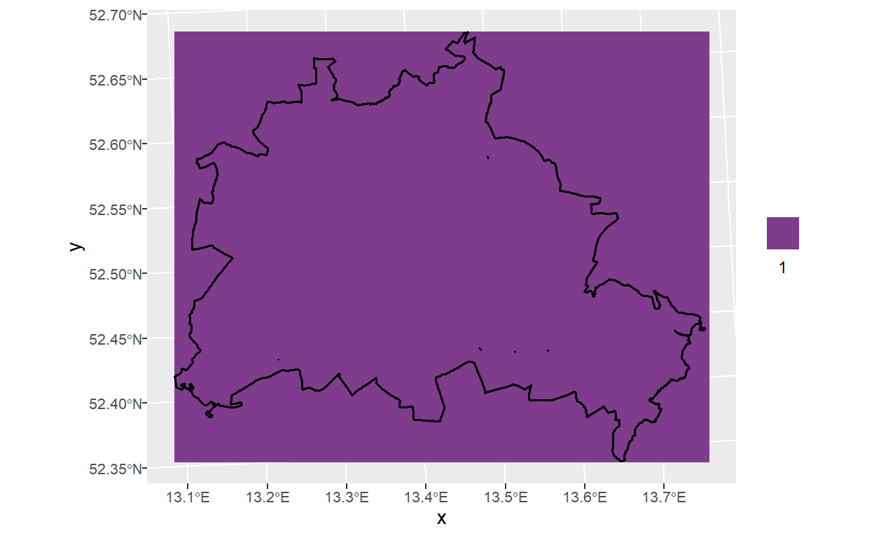

Expand Raster

Expand On All Sides

If you want to expand the raster (similar to a buffer around a polygon) you can just add cells to all sides. You can do this by adding an integer number in the y argument in the function extend of the {terra} package.

# expand the map
temp_exp_all <- terra::extend(x = temp, # template raster as input
                              y = 10, # number of cells to add
                              fill = 2) # value for new cells

# plot the map again
p2 <- d6geodata::plot_qualitative_map(temp_exp_all)
p2 + p_berlin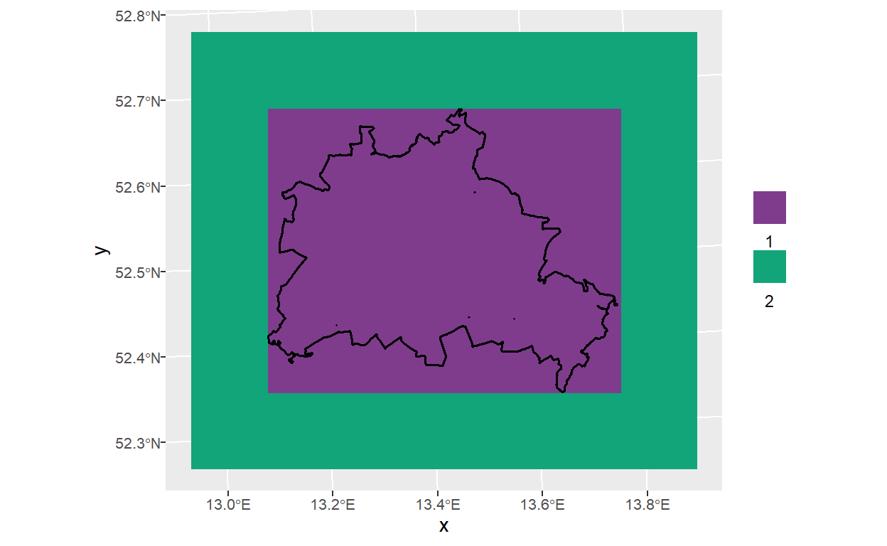

Expand On Two Sides

You can also expand the raster in one or two different directions only by adding cells on two opposite sides.

temp_exp_tb_sides <- terra::extend(x = temp,
                                   y = c(10, 0), # add 10 cells on top and below
                                   fill = 2,)
p3 <- d6geodata::plot_qualitative_map(temp_exp_tb_sides)
p3 + p_berlin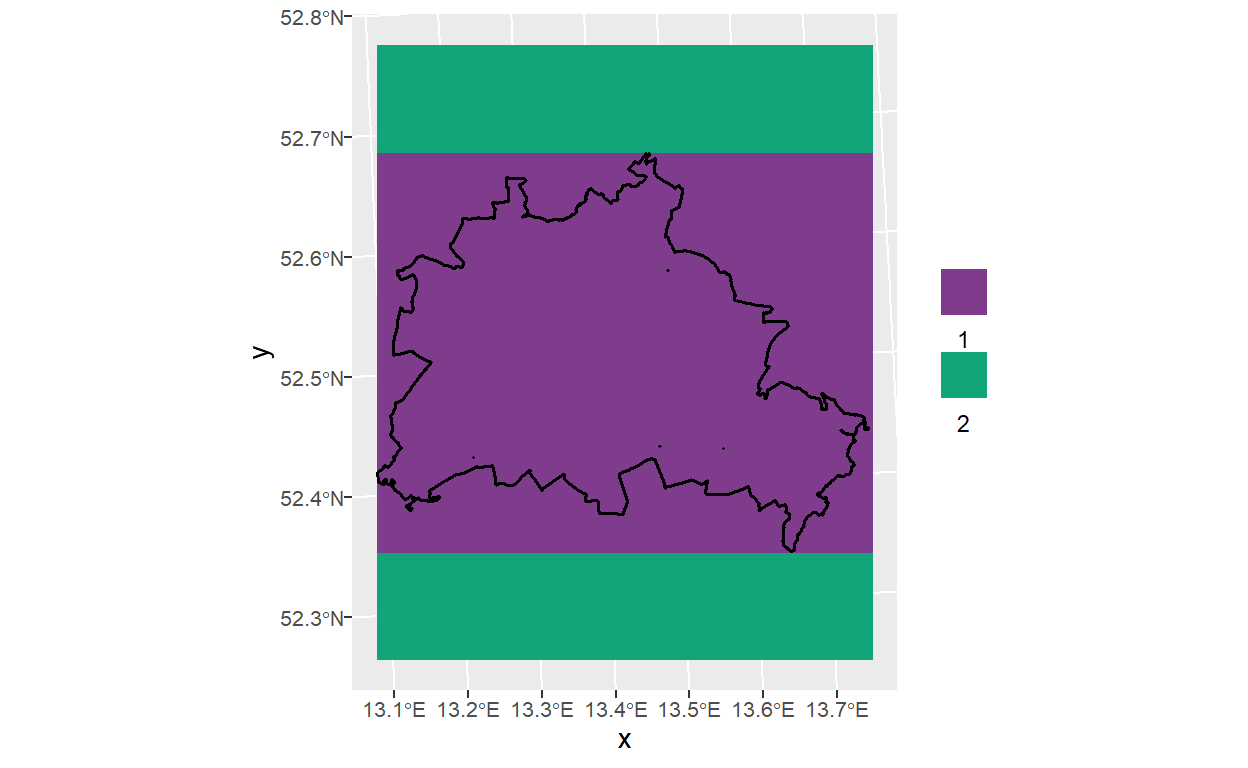

Expand On One Side With A Custom Extent

In this case we use a workaround by using a custom extent. Here we are adding cells on the left (western) side by using the xmin of the larger extend. Xmax, ymin, ymax are from the given extent.

temp_exp_1_sides <- terra::extend(x = temp,
                                  y = ext(ext(temp_exp_all)[1], # xmin
                                          ext(temp)[2], # xmax
                                          ext(temp)[3], # ymin
                                          ext(temp)[4]),# ymax
                                  fill = 2)

p4 <- d6geodata::plot_qualitative_map(temp_exp_1_sides)
p4 + p_berlin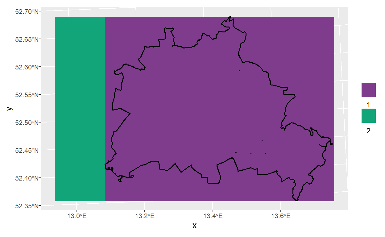

Combined Plot

Here you see a combination of all plots made to compare them directly.

# arrange plots in a 2x2 grid
(p1 + p_berlin + theme(legend.position="none") + p2 + p_berlin) / (p3 + p_berlin + p4 + p_berlin) + 
  plot_layout(guides = "collect") +
   plot_annotation(tag_levels = "1", tag_prefix = "(P", tag_suffix = ")") # add tag to every plot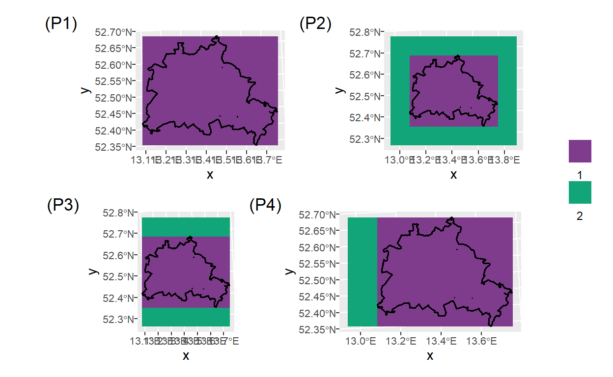

Rasterize Vector Data

With vect() you can make a spatVector (similar to a shapefile) from an extent object. Afterwards, we can use this spatVector to rasterize the data. This works similar with an sf object.

# create spatVector
temp_vec <- terra::vect(ext(temp), crs(temp)) # spatVector out of smallest raster extent

# rasterize spatVector
temp_rast <- rasterize(temp_vec, # vector data
                       temp_exp_all %>% disagg(10), 
                       # raster data with larger extent, disaggregated to 100m 
                       background = 2) # set to 2 to visualize the difference

temp_rast

class       : SpatRaster 
dimensions  : 570, 660, 1  (nrow, ncol, nlyr)
resolution  : 100, 100  (x, y)
extent      : 4521040, 4587040, 3243790, 3300790  (xmin, xmax, ymin, ymax)
coord. ref. : +proj=laea +lat_0=52 +lon_0=10 +x_0=4321000 +y_0=3210000 +ellps=GRS80 +units=m +no_defs 
source(s)   : memory
name        : layer 
min value   :     1 
max value   :     2 

Rasterized Plot

View the results.

d6geodata::plot_qualitative_map(temp_rast)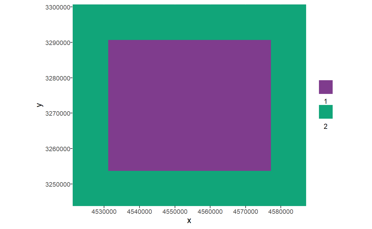

Extract With Vector Data

Imagine you have a track of an animal and you want to know what information lays in this track. In this case, you can use your line and extract the values from a raster below. There are several ways to this but the easiest way is to use the extract() function form the {terra} package to get the values laying under the vector data.

For this, you can use any vector data (points, lines, polygons) with the same projection and extent to extract values from a raster. The extract() function uses the raster as first input and the vector data as second. Depending on the type of data you are using you can define a function for the extraction like min, max or mean. ‘Cells’ gives you the call ID, ‘xy’ the coordinates and ‘ID’ the row number of your extraction. As mentioned, it is important that both the vector and the raster have the same projection.

Line For Extraction

For this we are just creating a dummy line with coordinates laying within the raster

# create points
pts <- tibble(x = c(4528790, 4576890), # a point out of two coordinates from the raster
              y = c(3271740, 3272140))

# create line from points
dummy_line <- st_as_sf(pts,             # a line made out of the point data
                       coords = c("x", "y"), # specify columns of xy coordinates
                       crs = st_crs(temp)$wkt, # using the same projection as for the template raster
                       sf_column_name = "geometry",
                       remove = FALSE) %>% 
  summarise(do_union = FALSE) %>% # this part is for creating the lines out of the points
  st_cast("LINESTRING") %>% # this as well
  mutate(id = 1:n()) # add an id

Plot Of Raster And Line

p5 <- d6geodata::plot_qualitative_map(temp_rast) + # first plot raster
  geom_sf(data = dummy_line)                       # plot line on top of the raster

p5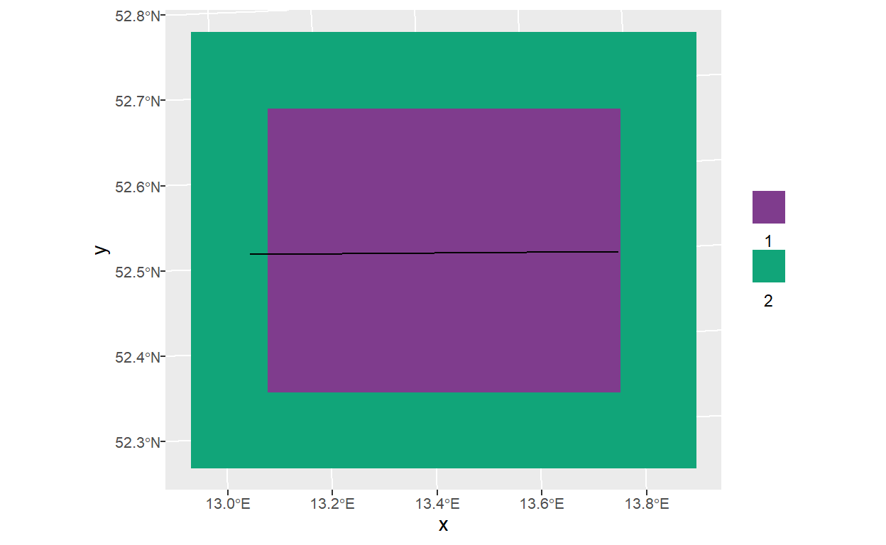

Extraction From Line

Here we finally extract the data and view the result with a table.

ext_tab <- terra::extract(x = temp_rast, # template raster as first input
               y = dummy_line, # dummy line as second input
               fun=NULL, # here you can set a function to summarise the data directly
               method="simple", 
               cells=FALSE, # here you can get the cell number as well if cell = TRUE
               xy=FALSE, # here the xy coordinates if xy = TRUE
               ID=TRUE # and the id in front of each row
               )

As you already can see on the plot, the largest part of the line lays within the purple area (value = 1). This function can be used to know on which land use class your track lays, for example.

table(ext_tab$layer)

  1   2 
463  23 

Visualize Data With Tidyterra

There are several ways to plot raster data with ggplot and one relatively new way is to do it with the package {tidyterra}. It has some well developed {ggplot} functions, but it cannot always be combined with the base functions of {ggplot}. If you use this package you may have to stay within the package functions.

library(tidyterra)

ggplot() + 
  geom_spatraster(data = temp_rast) + # use geom_spatraster() to plot the raster data with {tidyterra}
  p_berlin # add vector data of Berlin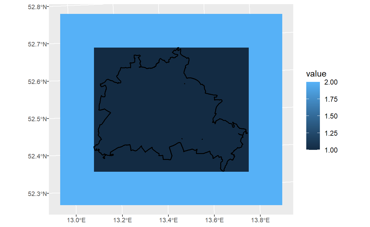

# same a before, but add some color to the plot
ggplot() + 
  geom_spatraster(data = temp_rast) +
  scale_fill_whitebox_c(palette = "purple") +
  p_berlin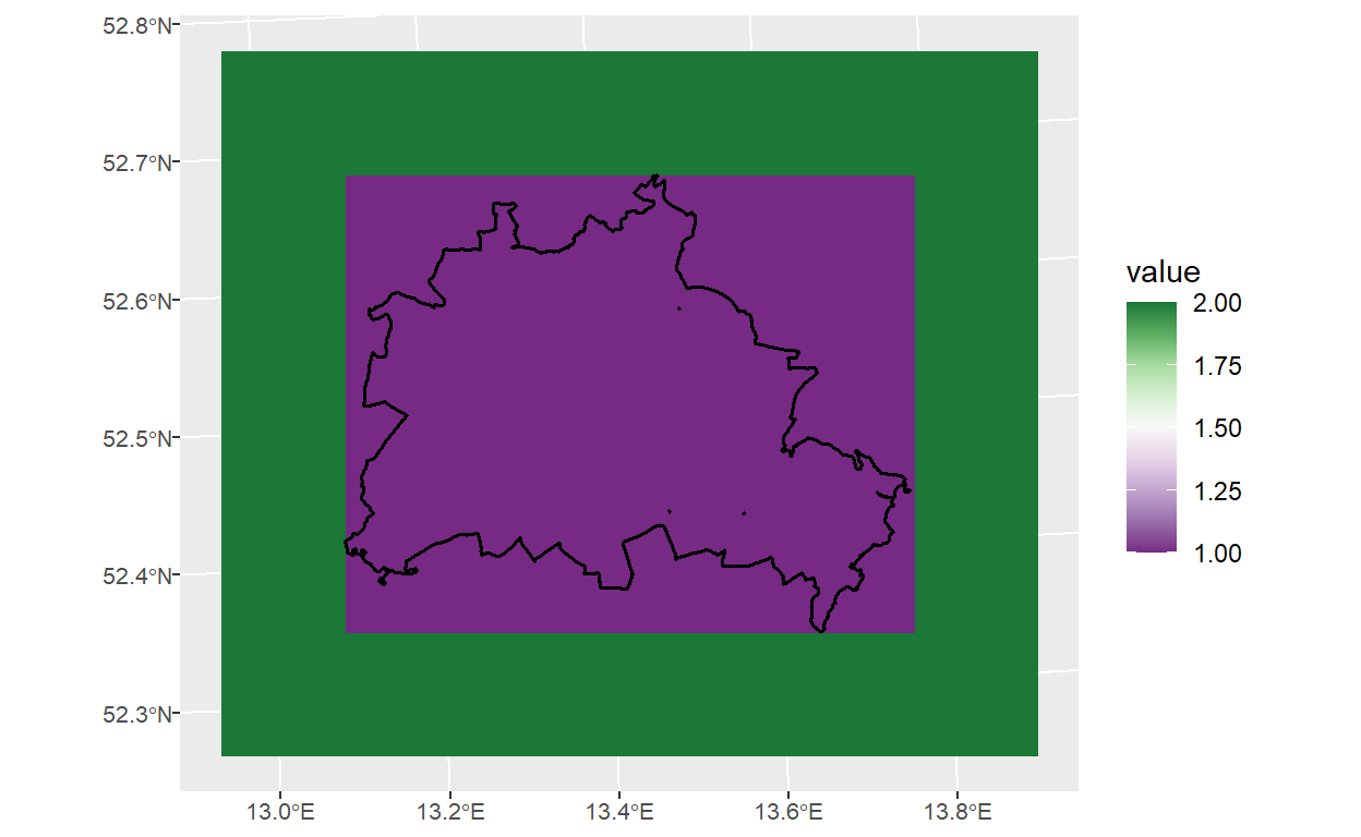

Summary

You learned how to extend a raster and how to extract data from a raster by using {sf} and {terra}. Of course there are several ways to do this, but this the most convenient way!!!