Preparation
To visualize the data sets, we use the {ggplot2} package. We will also use the {sf} and the {terra} packages to work and plot spatial data–vector and raster, respectively–in R. Make sure all packages are installed when running the code snippets.
# install.packages("ggplot2")
# install.packages("sf")
# install.packages("terra")

library(ggplot2)

### set "empty" theme with centered titles for ggplot output
theme_set(theme_void())
theme_update(plot.title = element_text(face = "bold", hjust = .5))
{rnaturalearth}
NaturalEarth is a public domain map data set that features vector and raster data of physical and cultural properties. It is available at 1:10m, 1:50m, and 1:110 million scales.
{rnaturalearth} is an R package to hold and facilitate interaction with NaturalEarth map data via dedicated ne_* functions. After loading the package, you can for example quickly access shapefiles of all countries–the resulting spatial object contains vector data that is already projected and can be stored as either sp or sf format:
## install development version of {rnaturalearth} as currently the
## download doesn't work in the CRAN package version
# install.packages("remotes")
# remotes::install_github("ropensci/rnaturalearth")

# if downloading raster data such as 'MRS_50m' is not working try to install the developer version of 'rnaturalearth' by using
# remotes::install_dev("rnaturalearth")

## for high resolution data, also install {rnaturalearthhires}
# remotes::install_github("ropensci/rnaturalearthhires")

library(rnaturalearth)

## store as sf object (simple features)
world <- ne_countries(returnclass = "sf")
class(world)
[1] "sf" "data.frame"sf::st_crs(world)[1]$input
[1] "WGS 84"Country Data
This country data set (which is actually not downloaded but stored locally by installing the package) already contains several useful variables, mostly referring to different naming conventions (helpful when joining with other data sets), to identify continents and regions, and also some information on population size, GDP, and economy:
names(world) [1] "featurecla" "scalerank" "labelrank" "sovereignt" "sov_a3"
[6] "adm0_dif" "level" "type" "tlc" "admin"
[11] "adm0_a3" "geou_dif" "geounit" "gu_a3" "su_dif"
[16] "subunit" "su_a3" "brk_diff" "name" "name_long"
[21] "brk_a3" "brk_name" "brk_group" "abbrev" "postal"
[26] "formal_en" "formal_fr" "name_ciawf" "note_adm0" "note_brk"
[31] "name_sort" "name_alt" "mapcolor7" "mapcolor8" "mapcolor9"
[36] "mapcolor13" "pop_est" "pop_rank" "pop_year" "gdp_md"
[41] "gdp_year" "economy" "income_grp" "fips_10" "iso_a2"
[46] "iso_a2_eh" "iso_a3" "iso_a3_eh" "iso_n3" "iso_n3_eh"
[51] "un_a3" "wb_a2" "wb_a3" "woe_id" "woe_id_eh"
[56] "woe_note" "adm0_iso" "adm0_diff" "adm0_tlc" "adm0_a3_us"
[61] "adm0_a3_fr" "adm0_a3_ru" "adm0_a3_es" "adm0_a3_cn" "adm0_a3_tw"
[66] "adm0_a3_in" "adm0_a3_np" "adm0_a3_pk" "adm0_a3_de" "adm0_a3_gb"
[71] "adm0_a3_br" "adm0_a3_il" "adm0_a3_ps" "adm0_a3_sa" "adm0_a3_eg"
[76] "adm0_a3_ma" "adm0_a3_pt" "adm0_a3_ar" "adm0_a3_jp" "adm0_a3_ko"
[81] "adm0_a3_vn" "adm0_a3_tr" "adm0_a3_id" "adm0_a3_pl" "adm0_a3_gr"
[86] "adm0_a3_it" "adm0_a3_nl" "adm0_a3_se" "adm0_a3_bd" "adm0_a3_ua"
[91] "adm0_a3_un" "adm0_a3_wb" "continent" "region_un" "subregion"
[96] "region_wb" "name_len" "long_len" "abbrev_len" "tiny"
[101] "homepart" "min_zoom" "min_label" "max_label" "label_x"
[106] "label_y" "ne_id" "wikidataid" "name_ar" "name_bn"
[111] "name_de" "name_en" "name_es" "name_fa" "name_fr"
[116] "name_el" "name_he" "name_hi" "name_hu" "name_id"
[121] "name_it" "name_ja" "name_ko" "name_nl" "name_pl"
[126] "name_pt" "name_ru" "name_sv" "name_tr" "name_uk"
[131] "name_ur" "name_vi" "name_zh" "name_zht" "fclass_iso"
[136] "tlc_diff" "fclass_tlc" "fclass_us" "fclass_fr" "fclass_ru"
[141] "fclass_es" "fclass_cn" "fclass_tw" "fclass_in" "fclass_np"
[146] "fclass_pk" "fclass_de" "fclass_gb" "fclass_br" "fclass_il"
[151] "fclass_ps" "fclass_sa" "fclass_eg" "fclass_ma" "fclass_pt"
[156] "fclass_ar" "fclass_jp" "fclass_ko" "fclass_vn" "fclass_tr"
[161] "fclass_id" "fclass_pl" "fclass_gr" "fclass_it" "fclass_nl"
[166] "fclass_se" "fclass_bd" "fclass_ua" "geometry" We can quickly plot it:
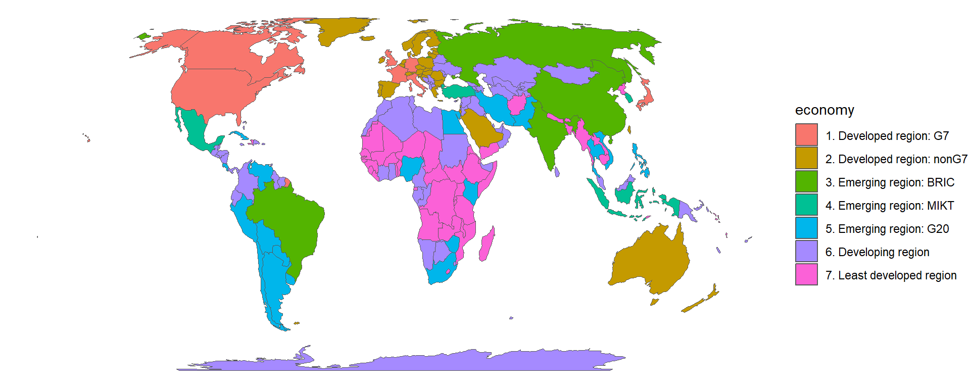
NOTE: Unfortunately, NaturalEarth is using weird de-facto and on-the-ground rules to define country borders which do not follow the borders the UN and most countries agree on. For correct and official borders, please use the {rgeoboundaries} package (see below).
Physical Data Sources
You can specify the scale, category, and type you want as in the examples below.
glacier_small <- ne_download(type = "glaciated_areas", category = "physical",
                             scale = "small", returnclass = "sf")

glacier_large <- ne_download(type = "glaciated_areas", category = "physical",
                             scale = "large", returnclass = "sf")
Now we can compare the impact of different scales specified–there is a notable difference in detail here (and also in size of the object with 11 versus 1886 observations).
ggplot() +
  geom_sf(data = world, color = "grey85", fill = "grey85") +
  geom_sf(data = glacier_small, color = "grey40", fill = "grey40") +
  coord_sf(crs = "+proj=eqearth")

ggplot() +
  geom_sf(data = world, color = "grey85", fill = "grey85") +
  geom_sf(data = glacier_large, color = "grey40", fill = "grey40") +
coord_sf(crs = "+proj=eqearth")library(patchwork)
small <- ggplot() +
geom_sf(data = world, color = "grey85", fill = "grey85", lwd = .05) +
geom_sf(data = glacier_small, color = "grey40", fill = "grey40") +
coord_sf(crs = "+proj=eqearth") +
labs(title = 'scale = "small"')
large <- ggplot() +
geom_sf(data = world, color = "grey85", fill = "grey85", lwd = .05) +
geom_sf(data = glacier_large, color = "grey40", fill = "grey40") +
coord_sf(crs = "+proj=eqearth") +
labs(title = 'scale = "large"')
small + large * theme(plot.margin = margin(0, -20, 0, -20))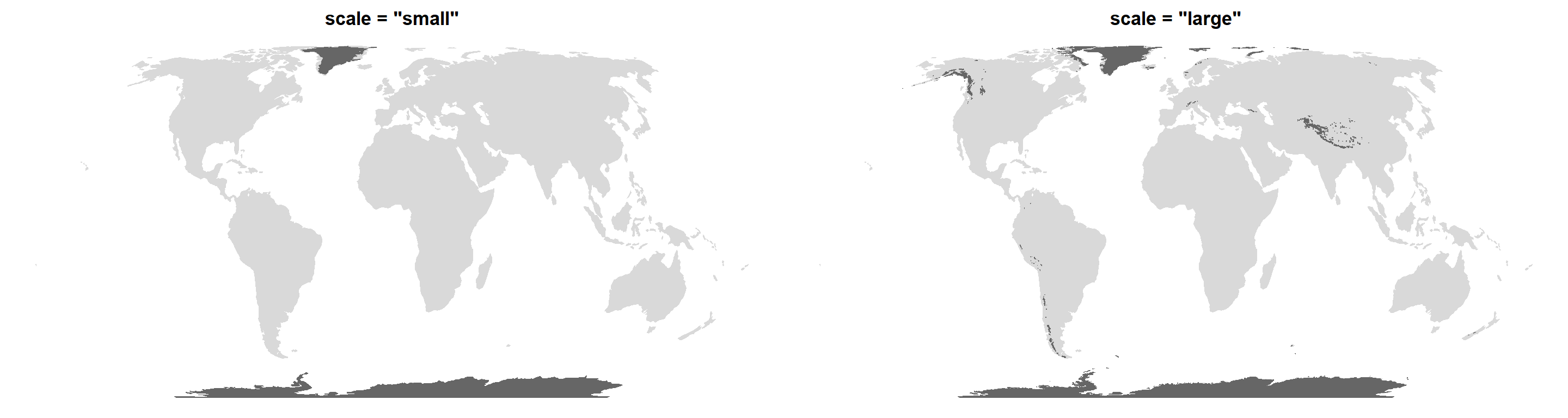
Cultural Data Sources
NaturalEarth also provides several cultural data sets, such as airports, roads, disputed areas. Let’s have a look at the urban areas across the world:
urban <- ne_download(type = "urban_areas", category = "cultural",
                     scale = "medium", returnclass = "sf")

ggplot() +
  geom_sf(data = world, color = "grey90", fill = "grey90") +
  geom_sf(data = urban, color = "firebrick", fill = "firebrick") +
  coord_sf(crs = "+proj=eqearth")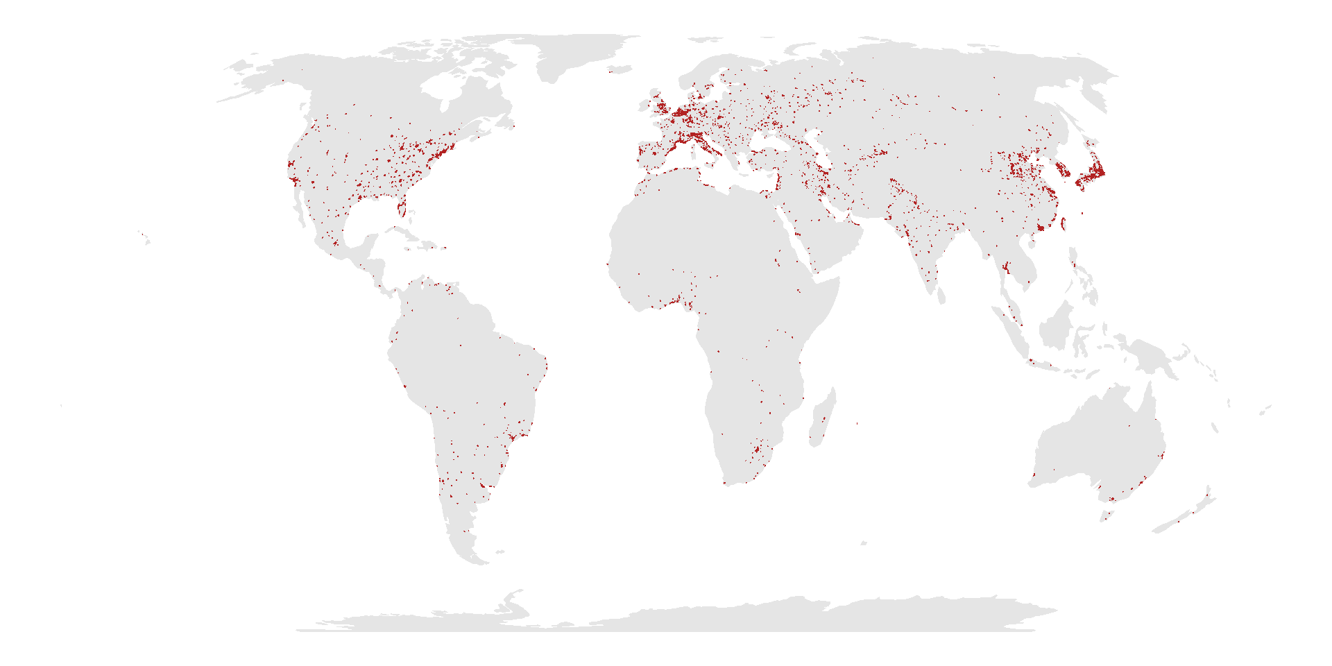
Relief Data
The physical and cultural data sets showcased above are all vector data. NaturalEarth also provides raster data, namely gridded relief data:
relief <- ne_download(type = "MSR_50M", category = "raster",
                      scale = 50, returnclass = "sf")

terra::plot(relief)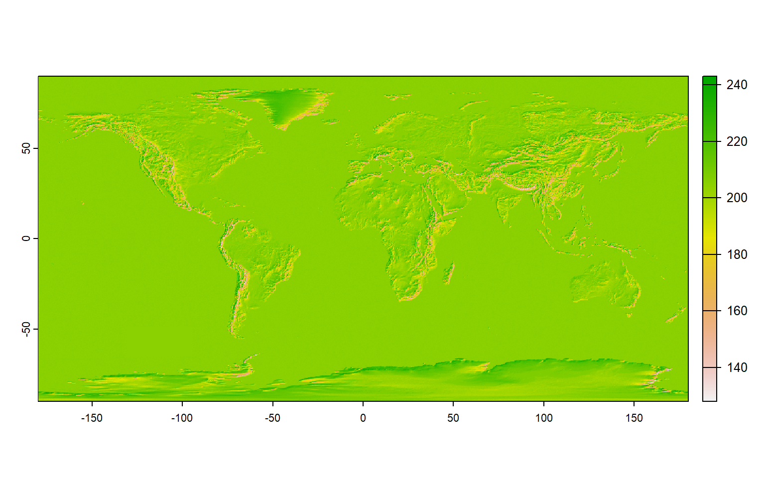
{rgeoboundaries}
The {rgeoboundaries} package uses the Global Database of Political Administrative Boundaries that provide generally accepted political borders. The data are licensed openly.
## install package from GitHub as it is not featured on CRAN yet
# install.packages("remotes")
# remotes::install_github("wmgeolab/rgeoboundaries")

library(rgeoboundaries)

gb_adm0()
Simple feature collection with 218 features and 3 fields
Geometry type: MULTIPOLYGON
Dimension: XY
Bounding box: xmin: -180 ymin: -90 xmax: 180 ymax: 83.63339
Geodetic CRS: WGS 84
First 10 features:
shapeGroup shapeType shapeName
1 AFG ADM0 Afghanistan
2 GBR ADM0 United Kingdom
3 ALB ADM0 Albania
4 DZA ADM0 Algeria
5 USA ADM0 United States
6 ATA ADM0 Antarctica
7 ATG ADM0 Antigua & Barbuda
8 ARG ADM0 Argentina
9 AND ADM0 Andorra
10 AGO ADM0 Angola
geometry
1 MULTIPOLYGON (((74.88986 37...
2 MULTIPOLYGON (((33.01302 34...
3 MULTIPOLYGON (((20.07889 42...
4 MULTIPOLYGON (((8.641941 36...
5 MULTIPOLYGON (((-168.1579 -...
6 MULTIPOLYGON (((-60.06171 -...
7 MULTIPOLYGON (((-62.34839 1...
8 MULTIPOLYGON (((-63.83417 -...
9 MULTIPOLYGON (((1.725802 42...
10 MULTIPOLYGON (((11.7163 -16...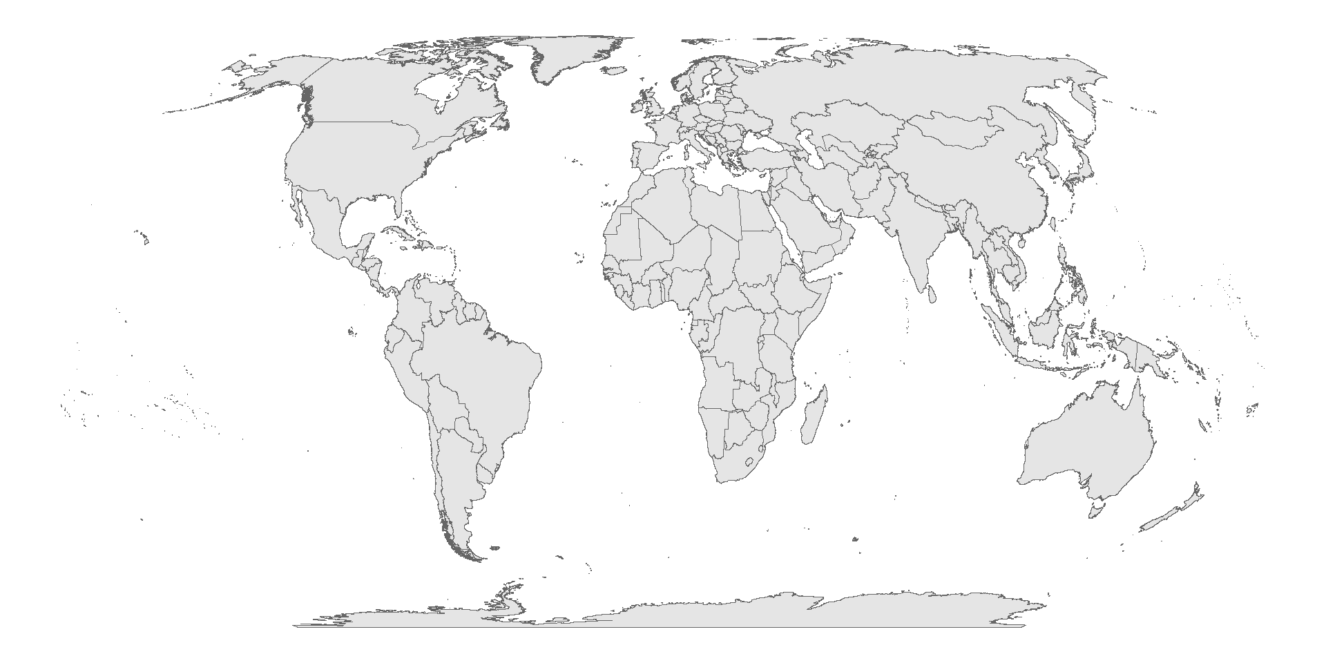
Lower administrative levels are available as well, e.g. in Germany adm1 represents federal states (“Bundesländer”), adm2 districts (“Kreise”) and so on.
Let’s plot the admin 1 levels for the DACH countries:
dach <- gb_adm1(c("germany", "switzerland", "austria"), type = "sscgs")

ggplot(dach) +
  geom_sf(aes(fill = shapeGroup)) +
  scale_fill_brewer(palette = "Set2")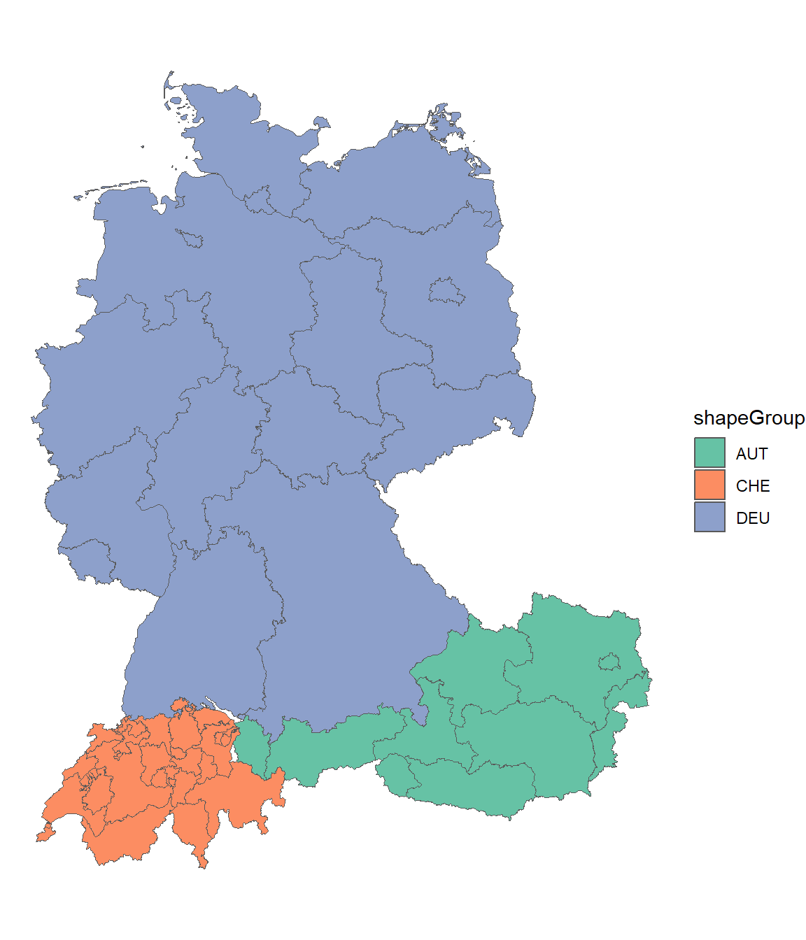
{osmdata}
OpenStreetMap (https://www.openstreetmap.org) is a collaborative project to create a free editable geographic database of the world. The geodata underlying the maps is considered the primary output of the project and is accessible from R via the {osmdata} package.
We first need to define our query and limit it to a region. You can explore the features and tags (also available as information via OpenStreetMap directly).
## install package
# install.packages("osmdata")

library(osmdata)

## explore features + tags
head(available_features())
[1] "4wd_only" "abandoned" "abutters" "access" "addr"
[6] "addr:city"head(available_tags("craft"))# A tibble: 6 × 2
Key Value
<chr> <chr>
1 craft agricultural_engines
2 craft atelier
3 craft bag_repair
4 craft bakery
5 craft basket_maker
6 craft beekeeper ## building the query, e.g. beekeepers
beekeeper_query <-
## you can automatically retrieve a boudning box (pr specify one manually)
getbb("Berlin") %>%
## build an Overpass query
opq(timeout = 999) %>%
## access particular feature
add_osm_feature("craft", "beekeeper")
## download data
sf_beekeepers <- osmdata_sf(beekeeper_query)Now we can investigate beekeepers in Berlin:
names(sf_beekeepers)[1] "bbox" "overpass_call" "meta"
[4] "osm_points" "osm_lines" "osm_polygons"
[7] "osm_multilines" "osm_multipolygons"head(sf_beekeepers$osm_points)Simple feature collection with 6 features and 27 fields
Geometry type: POINT
Dimension: XY
Bounding box: xmin: 13.24443 ymin: 52.35861 xmax: 13.69093 ymax: 52.573
Geodetic CRS: WGS 84
osm_id name addr:city addr:country addr:housenumber
358407135 358407135 <NA> <NA> <NA> <NA>
358407138 358407138 <NA> <NA> <NA> <NA>
417509803 417509803 <NA> <NA> <NA> <NA>
417509805 417509805 <NA> <NA> <NA> <NA>
597668310 597668310 <NA> <NA> <NA> <NA>
597668311 597668311 <NA> <NA> <NA> <NA>
addr:postcode addr:street addr:suburb check_date
358407135 <NA> <NA> <NA> <NA>
358407138 <NA> <NA> <NA> <NA>
417509803 <NA> <NA> <NA> <NA>
417509805 <NA> <NA> <NA> <NA>
597668310 <NA> <NA> <NA> <NA>
597668311 <NA> <NA> <NA> <NA>
contact:email contact:phone contact:website craft email
358407135 <NA> <NA> <NA> <NA> <NA>
358407138 <NA> <NA> <NA> <NA> <NA>
417509803 <NA> <NA> <NA> <NA> <NA>
417509805 <NA> <NA> <NA> <NA> <NA>
597668310 <NA> <NA> <NA> <NA> <NA>
597668311 <NA> <NA> <NA> <NA> <NA>
facebook instagram man_made opening_hours operator organic
358407135 <NA> <NA> <NA> <NA> <NA> <NA>
358407138 <NA> <NA> <NA> <NA> <NA> <NA>
417509803 <NA> <NA> <NA> <NA> <NA> <NA>
417509805 <NA> <NA> <NA> <NA> <NA> <NA>
597668310 <NA> <NA> <NA> <NA> <NA> <NA>
597668311 <NA> <NA> <NA> <NA> <NA> <NA>
phone product shop source website wheelchair works
358407135 <NA> <NA> <NA> <NA> <NA> <NA> <NA>
358407138 <NA> <NA> <NA> <NA> <NA> <NA> <NA>
417509803 <NA> <NA> <NA> <NA> <NA> <NA> <NA>
417509805 <NA> <NA> <NA> <NA> <NA> <NA> <NA>
597668310 <NA> <NA> <NA> <NA> <NA> <NA> <NA>
597668311 <NA> <NA> <NA> <NA> <NA> <NA> <NA>
geometry
358407135 POINT (13.69068 52.35918)
358407138 POINT (13.69093 52.35894)
417509803 POINT (13.68991 52.35888)
417509805 POINT (13.6902 52.35861)
597668310 POINT (13.24445 52.573)
597668311 POINT (13.24443 52.57295)beekeper_locations <- sf_beekeepers$osm_points
## Berlin borders via {geoboundaries}
sf_berlin <- gb_adm1(c("germany"), type = "sscgs")[6,] # the sixth element is Berlin
## Berlin border incl. district borders via our {d6berlin}
# remotes::install_github("EcoDynIZW/d6berlin")
sf_berlin <- d6berlin::sf_districts
ggplot(beekeper_locations) +
geom_sf(data = sf_berlin, fill = "grey10", color = "grey30") +
geom_sf(size = 4, color = "#FFB000", alpha = .3) +
labs(title = "Beekeepers in Berlin",
caption = "© OpenStreetMap contributors")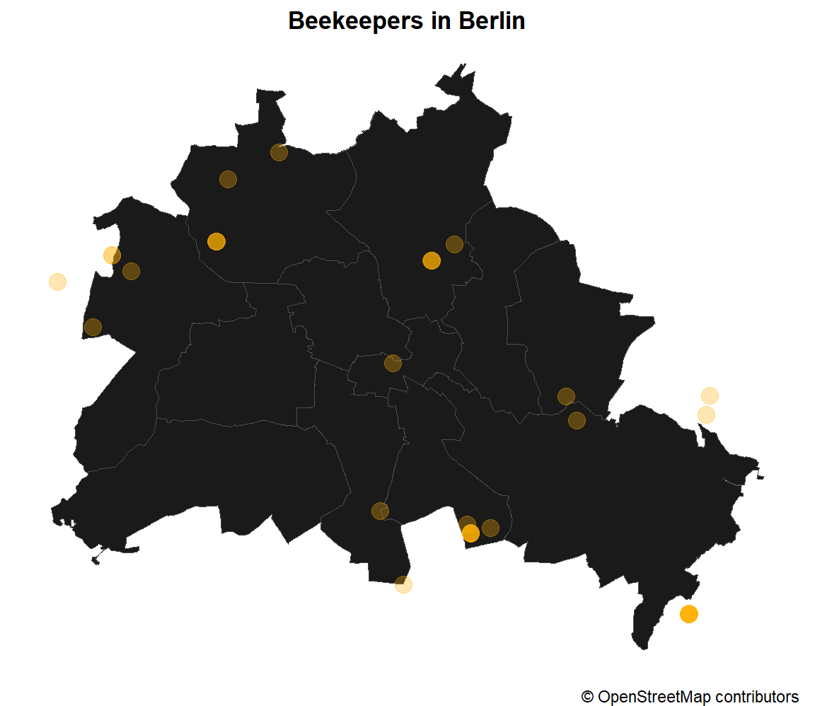
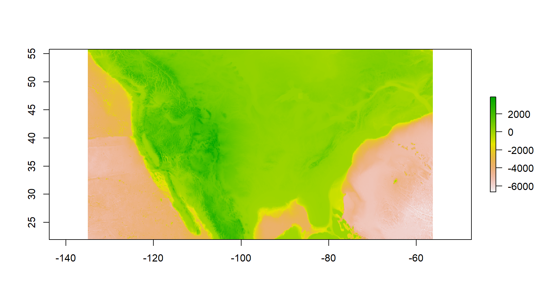
{elevatr}
The {elevatr} (https://github.com/jhollist/elevatr/) is an R package that provides access to elevation data from AWS Open Data Terrain Tiles and the Open Topography Global data sets API for raster digital elevation models (DEMs).
We first need to define a location or bounding box for our elevation data. This can either be a data frame or a spatial object. We use an sf object which holds the projection to be used when assessing the elevation data:
## install package
# install.packages("elevatr")

library(elevatr)

## manually specify corners of the bounding box of the US
bbox_usa <- data.frame(x = c(-125.0011, -66.9326),
                       y = c(24.9493, 49.5904))

## turn into spatial, projected bounding box
sf_bbox_usa <- sf::st_as_sf(bbox_usa, coords = c("x", "y"), crs = 4326)
Now we can download the elevation data with a specified resolution z (ranging from 1 to 14 with 1 being very coarse and 14 being very fine).
elev_usa <- get_elev_raster(locations = sf_bbox_usa, z = 5)

terra::plot(elev_usa)