Manage Spatial Data from Our Geodata Archive

Learn how to use the {d6geodata} R package that provides functions for accessing data from the Geodata archive of the Department of Ecological Dynamics. The two functions geo_overview() and get_geodata() are the main components for all members of our Department. Several other functions are within this package but only meant to be used by the Geodata Manager of the Department.

The {d6geodata} package aims to access the data from the Geodata archive of the EcoDyn Department for members only!

The two main functions are:

• geo_overview()
• get_geodata()

## remotes::install_github("EcoDynIZW/d6geodata")
## library(d6geodata)

If you want to work with geodata that is already stored in our Geodata archive you have two options:

1. Go to the EcoDynIZW Website, click on wikis and select Geodata. There you find several spatial data sets with respective metadaat and visualizations. In the metadata section, you’ll find the information . To donwload the data, cope the folder_name information provided in the metadata and use it as an input in the get_geodata() function from our {d6geodata} to get the data from our PopDynCloud. Another option is the function called geo_overview(). There you can select which data and from which location you want to have a list of data.

If you run the function geo_overview you have to decide if you want to see the raw or processed data by typing 1 for raw and 2 for processed data. Afterwards, you have to decide if you want to see the main (type 1) folders (the regions or sub-regions we have data from) or the sub (type 2) folders (the actually data we have in each region).

Example 1: Main Folder

d6geodata::geo_overview(path_to_cloud = "E:/PopDynCloud")
Raw or processed data: 

1: raw
2: processed

Auswahl: 2
choose folder type: 

1: main
2: sub

Auswahl: 1
[1] "atlas" "BB_MV_B" "berlin" "europe" "germany" "world"

Example 2: Sub Folder

d6geodata::geo_overview(path_to_cloud = "E:/PopDynCloud")
Raw or processed data: 

1: raw
2: processed

Auswahl: 2
choose folder type: 

1: main
2: sub

Auswahl: 2
$atlas
[1] "distance-to-human-settlements_atlas_2009_1m_03035_tif"
[2] "distance-to-kettleholes_atlas_2022_1m_03035_tif"      
[3] "distance-to-rivers_atlas_2009_1m_03035_tif"           
[4] "distance-to-streets_atlas_2022_1m_03035_tif"          
[5] "landuse_atlas_2009_1m_03035_tif"                      

$BB_MV_B
[1] "_archive" "_old_not_verified" "dist_path_bb_agroscapelabs"
[4] "scripts"                   

$berlin
 [1] "_old_not_verified"                            
 [2] "corine_berlin_2015_20m_03035_tif"            
 [3] "distance-to-paths_berlin_2022_100m_03035_tif" 
 [4]  "green-capacity_berlin_2020_10m_03035_tif"    
 [5] "imperviousness_berlin_2018_10m_03035_tif"     
 [6]  "light-pollution_berlin_2021_100m_03035_tif"  
 [7] "light-pollution_berlin_2021_10m_03035_tif"    
 [8]  "motorways_berlin_2022_100m_03035_tif"        
 [9] "noise-day-night_berlin_2017_10m_03035_tif"    
[10]  "population-density_berlin_2019_10m_03035_tif"
[11] "template-raster_berlin_2018_10m_03035_tif"    
[12] "tree-cover-density_berlin_2018_10m_03035_tif"

$europe
[1] "imperviousness_europe_2018_10m_03035_tif"

$germany
 [1] "_old_not_verified"                                          
 [2] "distance-to-motorway-rural-road_germany_2022_100m_03035_tif"
 [3] "distance-to-motorways_germany_2022_100m_03035_tif"          
 [4] "distance-to-paths_germany_2022_100m_03035_tif"              
 [5] "distance-to-roads-paths_germany_2022_100m_03035_tif"        
 [6] "distance-to-roads_germany_2022_100m_03035_tif"              
 [7] "distance_to_paths_germany_2022_100m_03035_tif"              
 [8] "motoroways_germany_2022_03035_osm_tif"                      
 [9] "motorway-rural-road_germany_2022_100m_03035_tif"            
[10] "motorways_germany_2022_100m_03035_tif"                      
[11] "paths_germany_2022_100m_03035_tif"                          
[12] "Roads-germany_2022_100m_03035_tif"                          
[13] "roads_germany_2022_100m_03035_tif"                          
[14] "tree-cover-density_germany_2015_100m_03035_tif"             

$world
character(0)

Now you can copy the name of one of the layers and paste it into the get_geodata() function

corine <-
  d6geodata::get_geodata(
    data_name = "corine_berlin_2018_20m_03035_tif",
    path_to_cloud = "E:/PopDynCloud",
    download_data = FALSE
  )

If you set download_data = TRUE the data will be download and copied to your data-raw folder. If the data-raw folder doesn’t exist, it will be created.

If you want to download more than one file, you can simply use lapply() and add multiple file names like this:

data_list <-
  lapply(
    c(
      "corine_berlin_2018_20m_03035_tif",
      "motorways_berlin_2022_100m_03035_tif"
    ),
    FUN = function(x) {
      d6geodata::get_geodata(
        data_name = x,
        path_to_cloud = "E:/PopDynCloud",
        download_data = FALSE
      )})

Additional functions

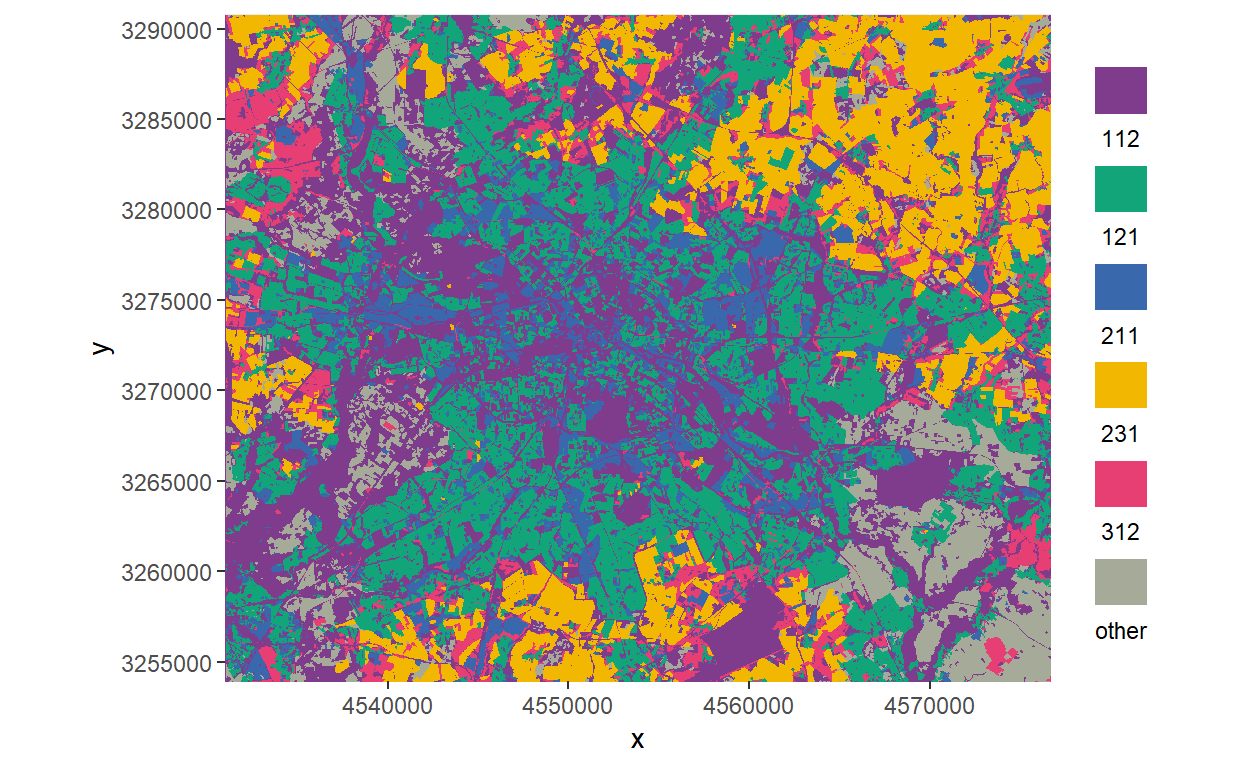
The three functions plot_binary_map(), plot_qualitative_map() and plot plot_quantitative_map() can be used to plot raster data with the respective color schemes we used for the Geodata wiki page (note that this function works only for raster data).

plot_binary_map(tif = tif)
plot_qualitative_map(tif = tif)
plot_quantitative_map(tif = tif)

Example plot

library(d6geodata)
plot_qualitative_map(tif = corine)