Ecological Dynamics: Spatial Datasets and Template Maps for Berlin

Cedric Scherer

The {d6berlin} package aims provide template maps for Berlin with carefully chosen and aesthetically pleasing defaults. Template maps include green spaces, imperviousness levels, water bodies, district borders, roads, and railways, plus the utility to add a globe with locator pin, a scalebar, and a caption to include the data sources.

There are two main functionalities:

Create a template map with imperviousness and green spaces with base_map_imp()
Provide various ready-to-use Berlin data sets with sf_*

Furthermore, the package provides utility to add a globe with locator pin, a scalebar, and a caption to include the data sources.

Installation

You can install the {d6berlin} package from GitHub:

## install.packages("remotes")
## remotes::install_github("EcoDynIZW/d6berlin")
library(d6berlin)

Note: If you are asked if you want to update other packages either press “No” (option 3) and continue or update the packages before running the install command again.

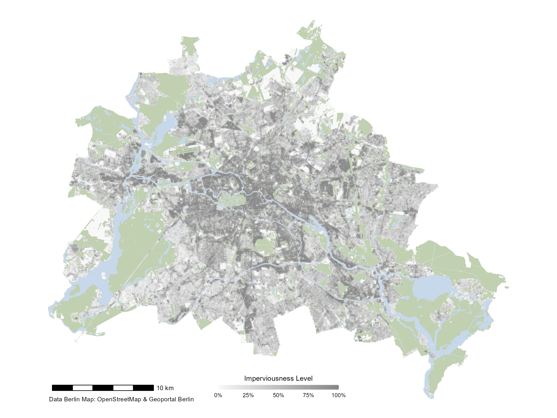
A Basic Template Map of Imperviousness

The basic template map shows levels of imperviousness and green areas in Berlin. The imperviousness raster data was derived from Geoportal Berlin (FIS-Broker) with a resolution of 10m. The vector data on green spaces was collected from data provided by the OpenStreetMap Contributors. The green spaces consist of a mixture of land use and natural categories (namely “forest”, “grass”, “meadow”, “nature_reserve”, “scrub”, “heath”, “beach”, “cliff”).

The map is projected in EPSG 4326 (WGS84).

d6berlin::base_map_imp()

#> Aggregating raster data.
#> Plotting basic map.
#> Styling map.

You can also customize the arguments, e.g. change the color intensity, add a globe with a locator pin, change the resolution of the raster, and move the legend to a custom position:

base_map_imp(color_intensity = 1, globe = TRUE, resolution = 500,
             legend_x = .17, legend_y = .12)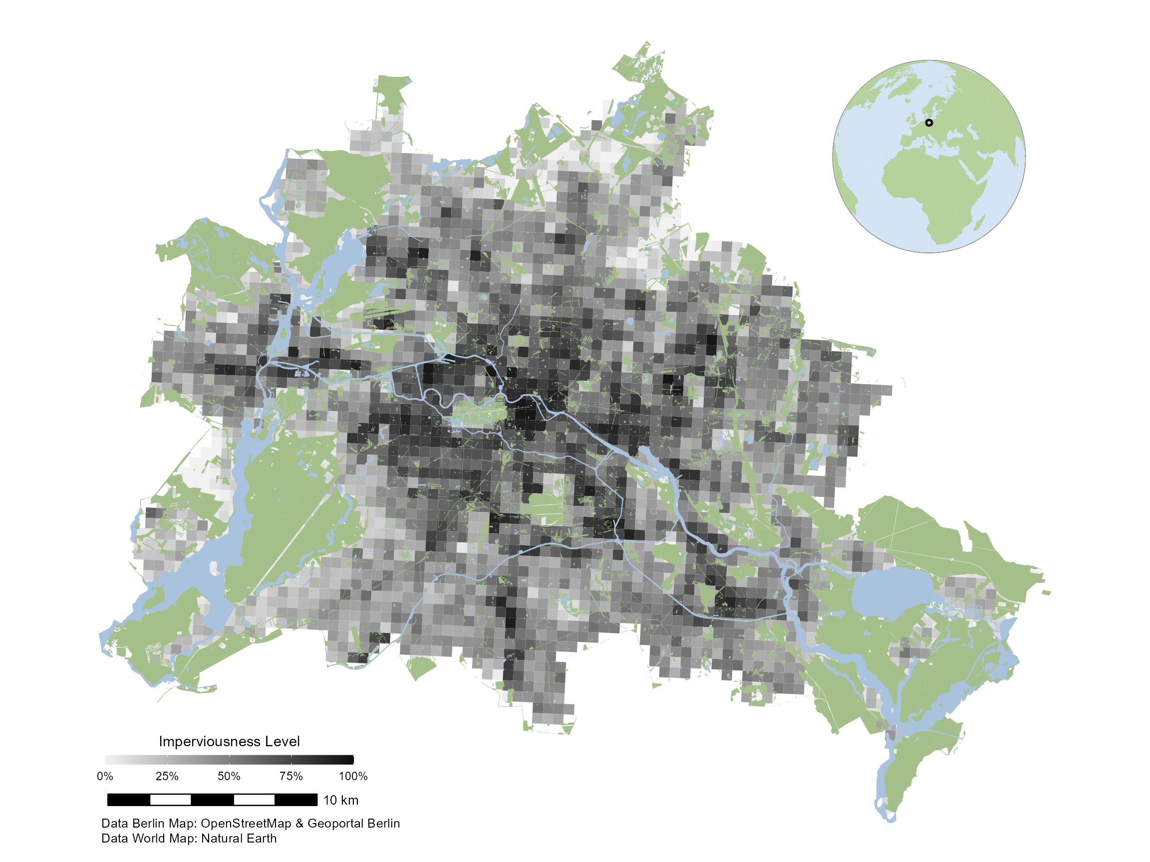

If you think the legend is not need, there is also an option called "none". (The default is "bottom". You can also use of the predefined setting "top" as illustrated below or a custom position as shown in the previous example.)

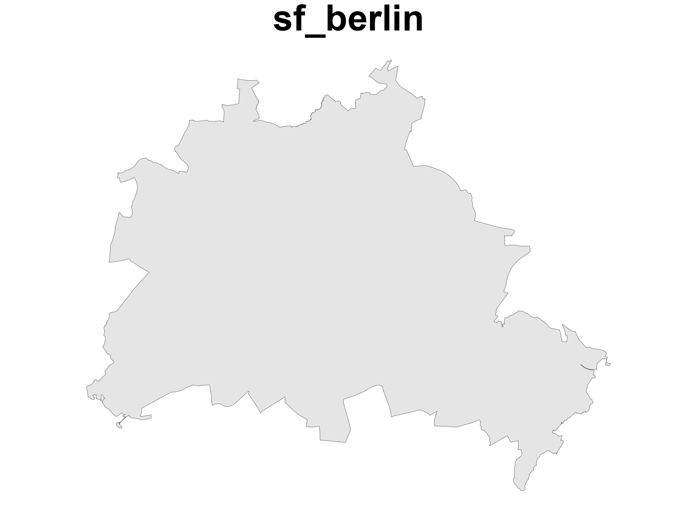
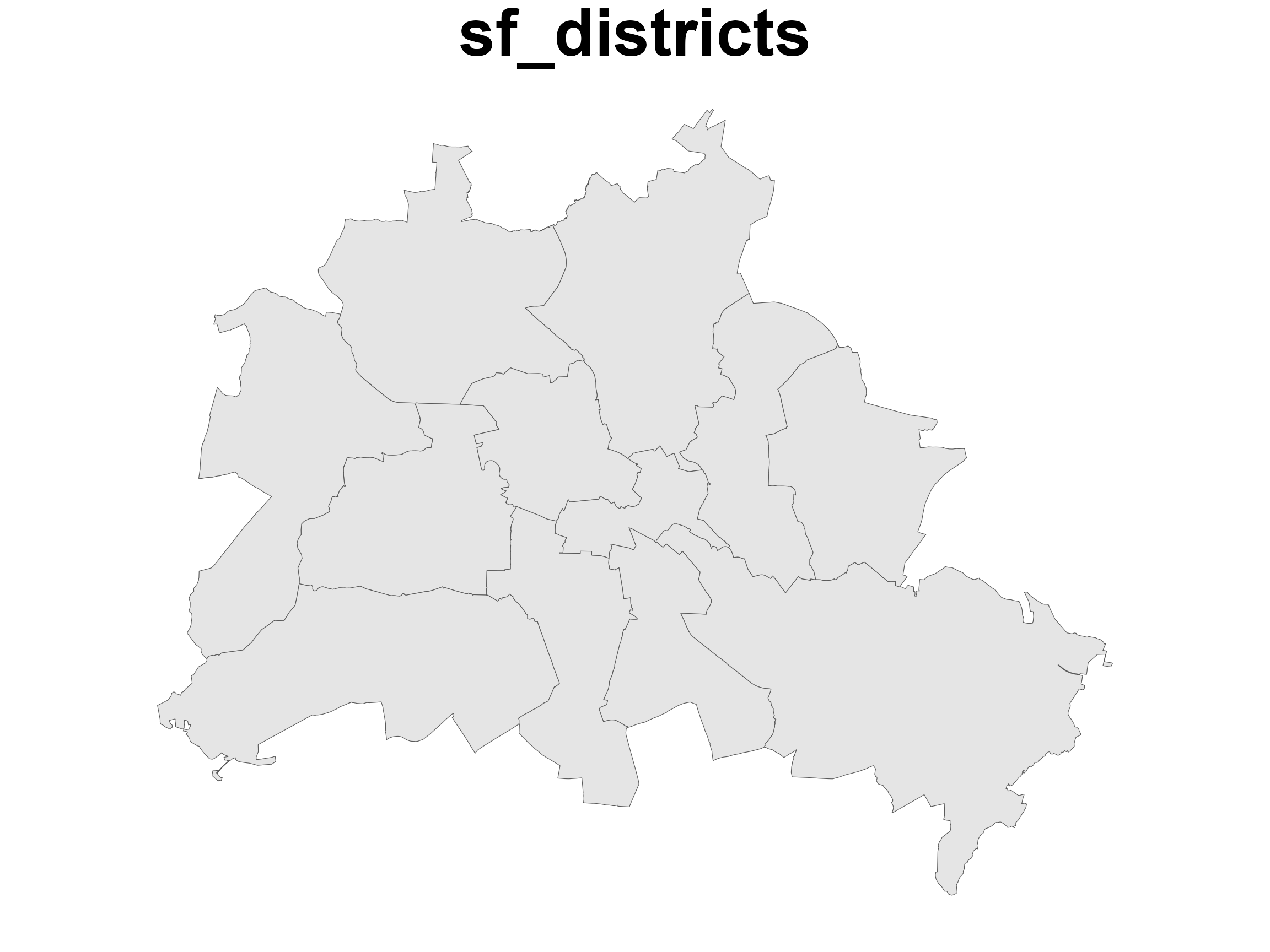
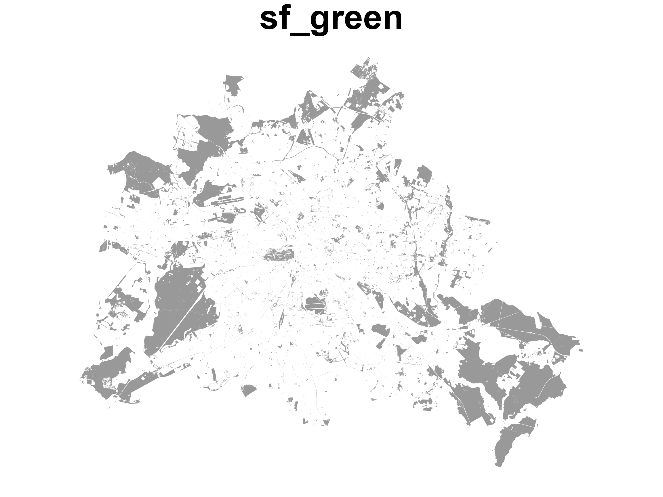
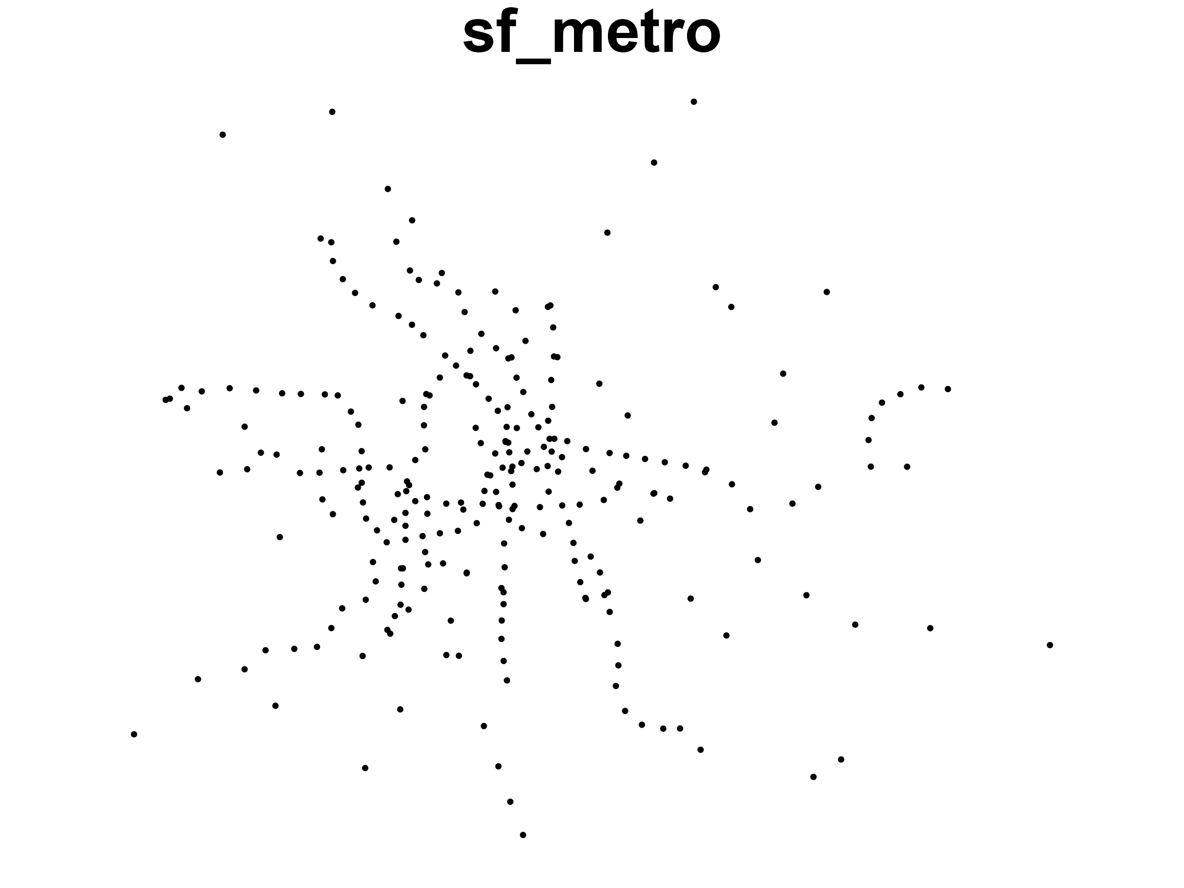
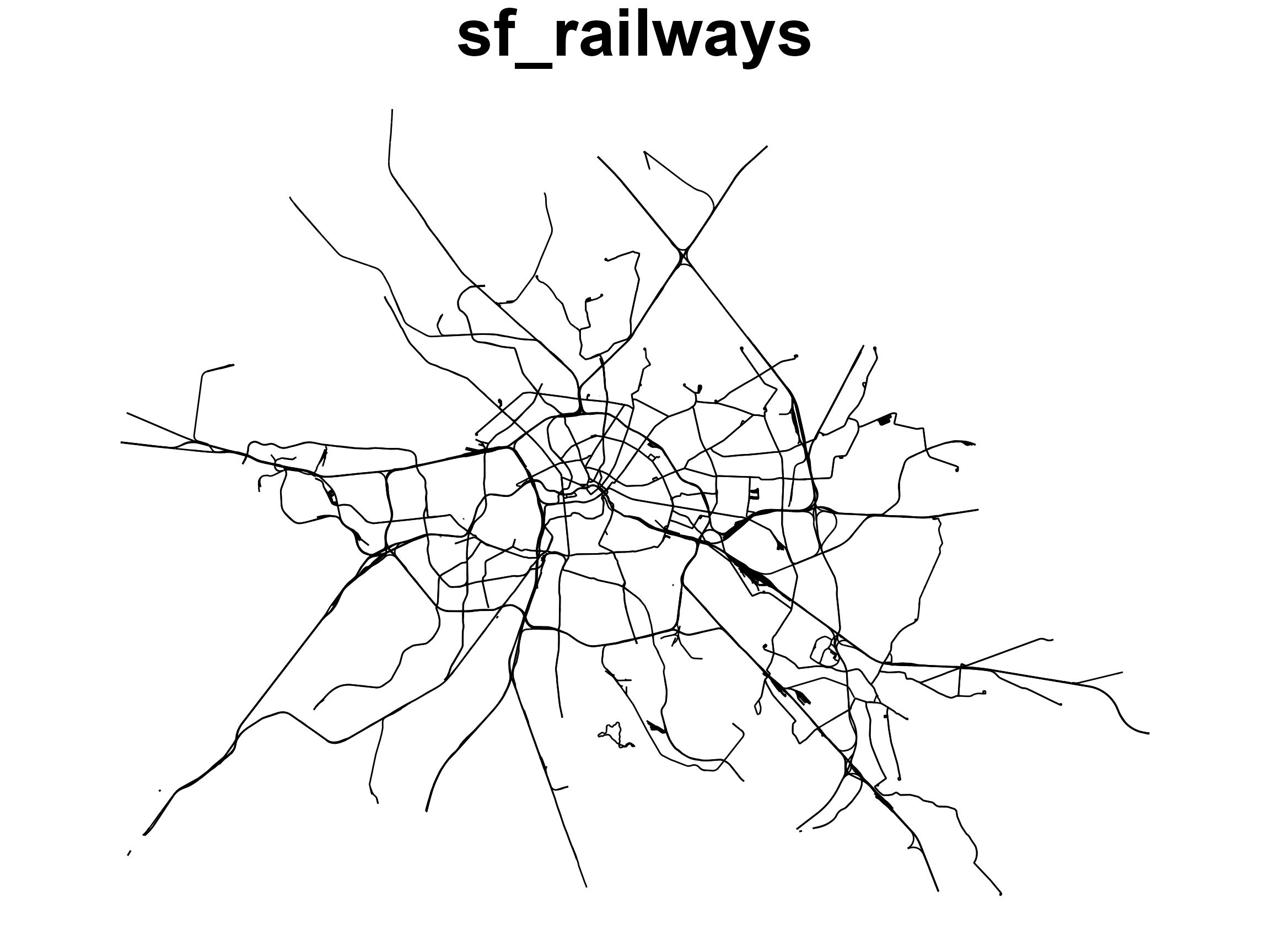
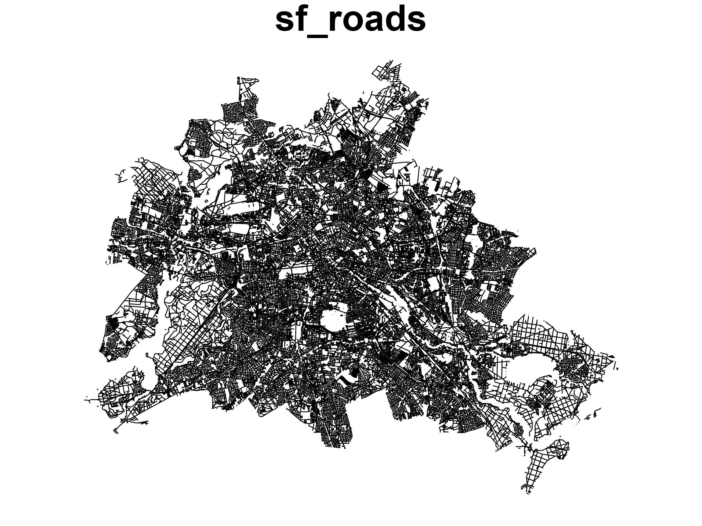
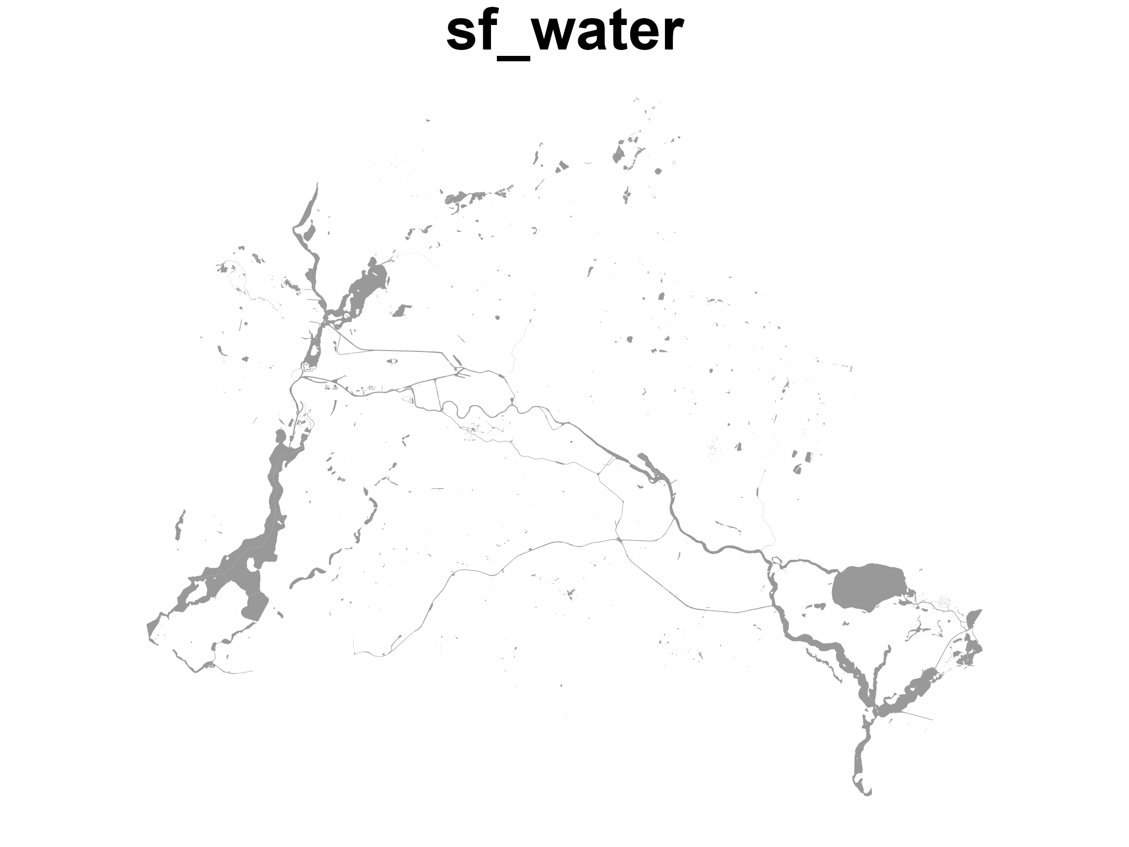
Berlin Data Sets

The package contains several data sets for Berlin. All of them start with sf_, e.g. d6berlin::sf_roads. Here is a full overview of the data sets that are available:

Adding Locations to the Map

Let’s assume you have recorded some animal locations or you want to plot another information on to of this plot. For example, let’s visualize the Berlin metro stations by adding geom_sf(data = x) to the template map:

library(ggplot2)
library(sf)

map <- base_map_imp(color_intensity = .4, resolution = 500, legend = "top")

map + geom_sf(data = sf_metro) ## sf_metro is contained in the {d6berlin} package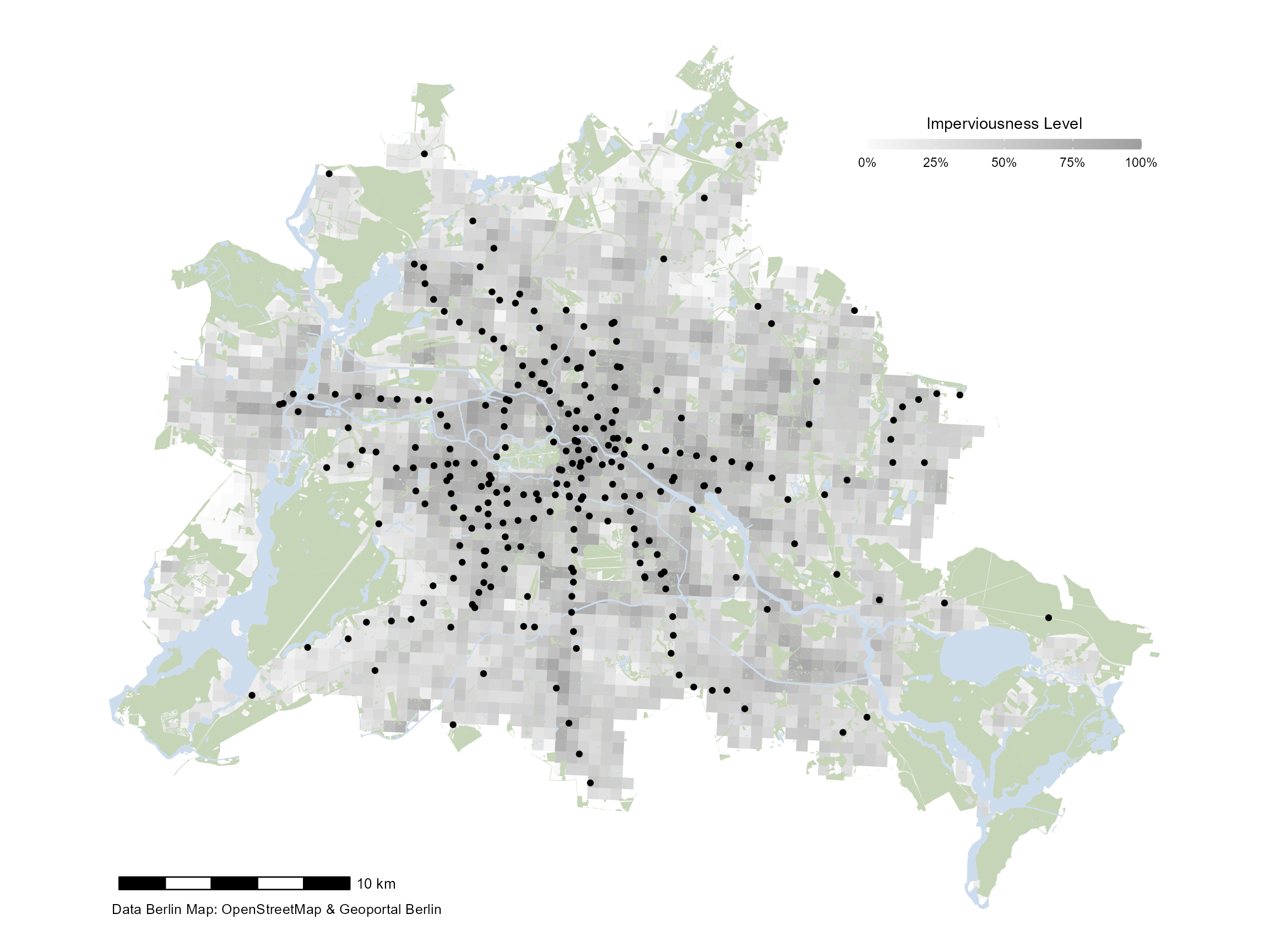

Note: Since the template map contains many filled areas, we recommend to add geometries with variables mapped to color|colour|col to the template maps.

You can, of course, style the appearance of the points as usual:

map + geom_sf(data = sf_metro, shape = 8, color = "red", size = 2)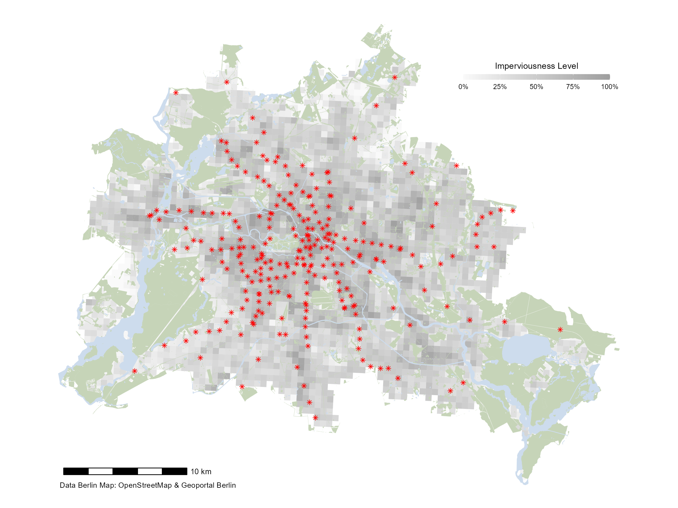

It is also possible to filter the data inside the geom_sf function — no need to use subset:

library(dplyr) ## for filtering
library(stringr) ## for filtering based on name

map + 
  geom_sf(data = filter(sf_metro, str_detect(name, "^U")), 
          shape = 21, fill = "dodgerblue", size = 2) +
  geom_sf(data = filter(sf_metro, str_detect(name, "^S")), 
          shape = 21, fill = "forestgreen", size = 2)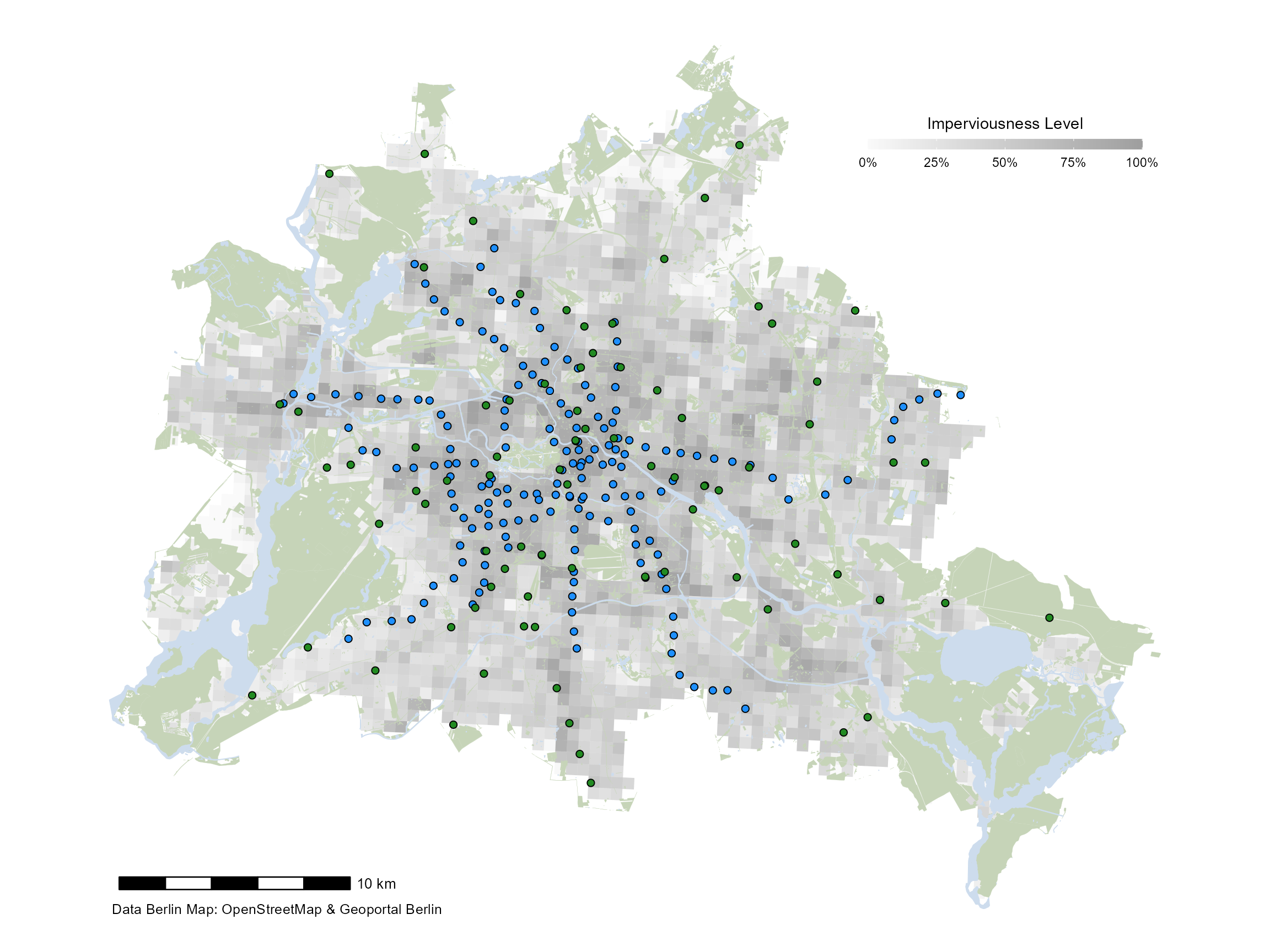

You can also use the mapping functionality of ggplot2 to address variables from your data set.

map + 
  geom_sf(data = sf_metro, aes(color = type), size = 2) +
  scale_color_discrete(type = c("forestgreen", "dodgerblue"), 
                       name = NULL) +
  guides(color = guide_legend(direction = "horizontal",
                              title.position = "top", 
                              title.hjust = .5))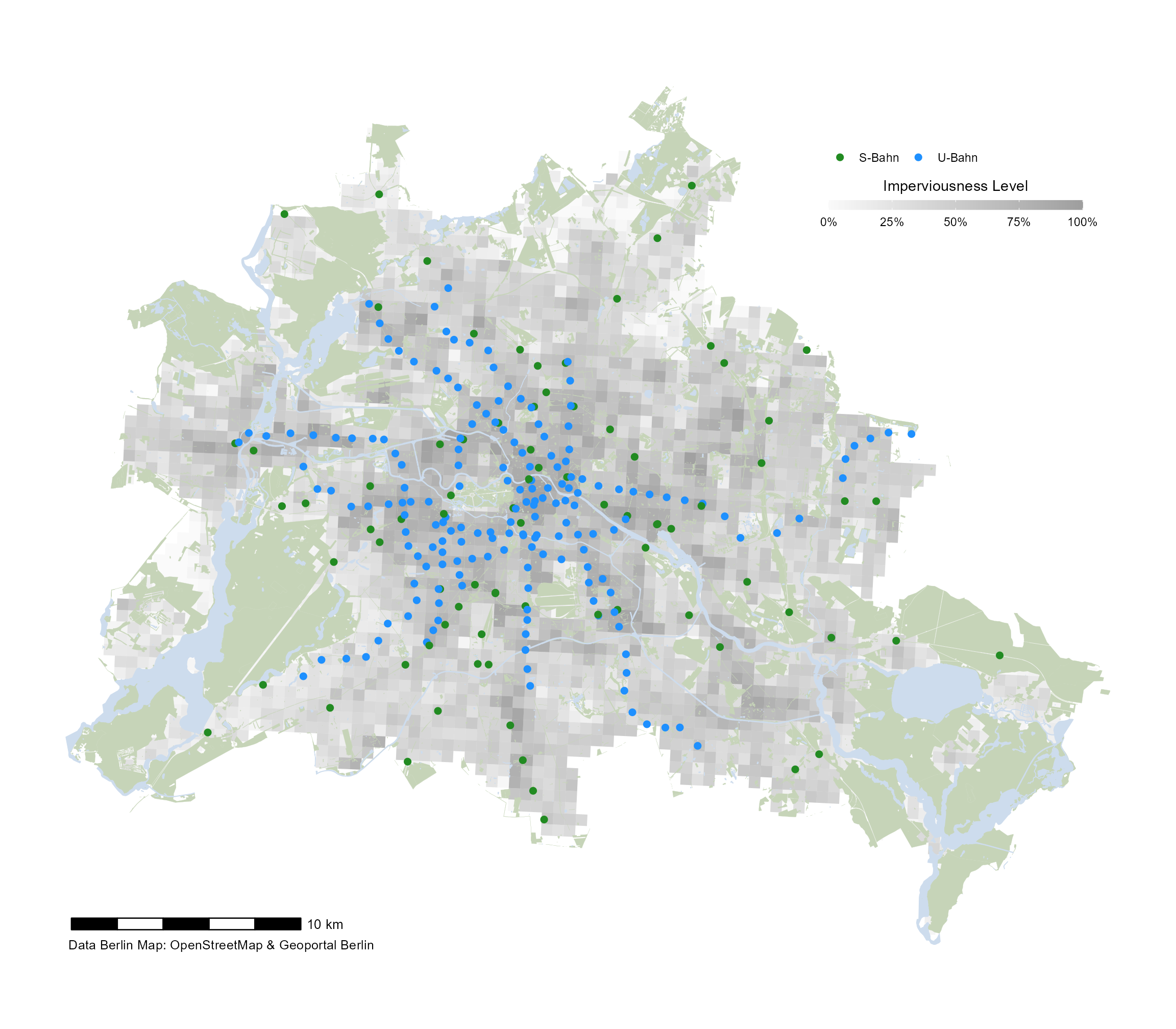

(It looks better if you style the legend in the same horizontal layout.)

Custom Styling

Since the output is a ggplot object, you can manipulate the result as you like (but don’t apply a new theme, this will mess up the legend design):

library(systemfonts) ## for title font

base_map_imp(color_intensity = 1, resolution = 250, globe = TRUE,
             legend_x = .17, legend_y = .12) + 
  geom_sf(data = sf_metro, shape = 21, fill = "white", 
          stroke = .4, size = 4) +
  ggtitle("Metro Stations in Berlin") + 
  theme(plot.title = element_text(size = 30, hjust = .5, family = "Bangers"),
        panel.grid.major = element_line(color = "white", linewidth = .3),
        axis.text = element_text(color = "black", size = 8),
        plot.background = element_rect(fill = "#fff0de", color = NA),
        plot.margin = margin(rep(20, 4)))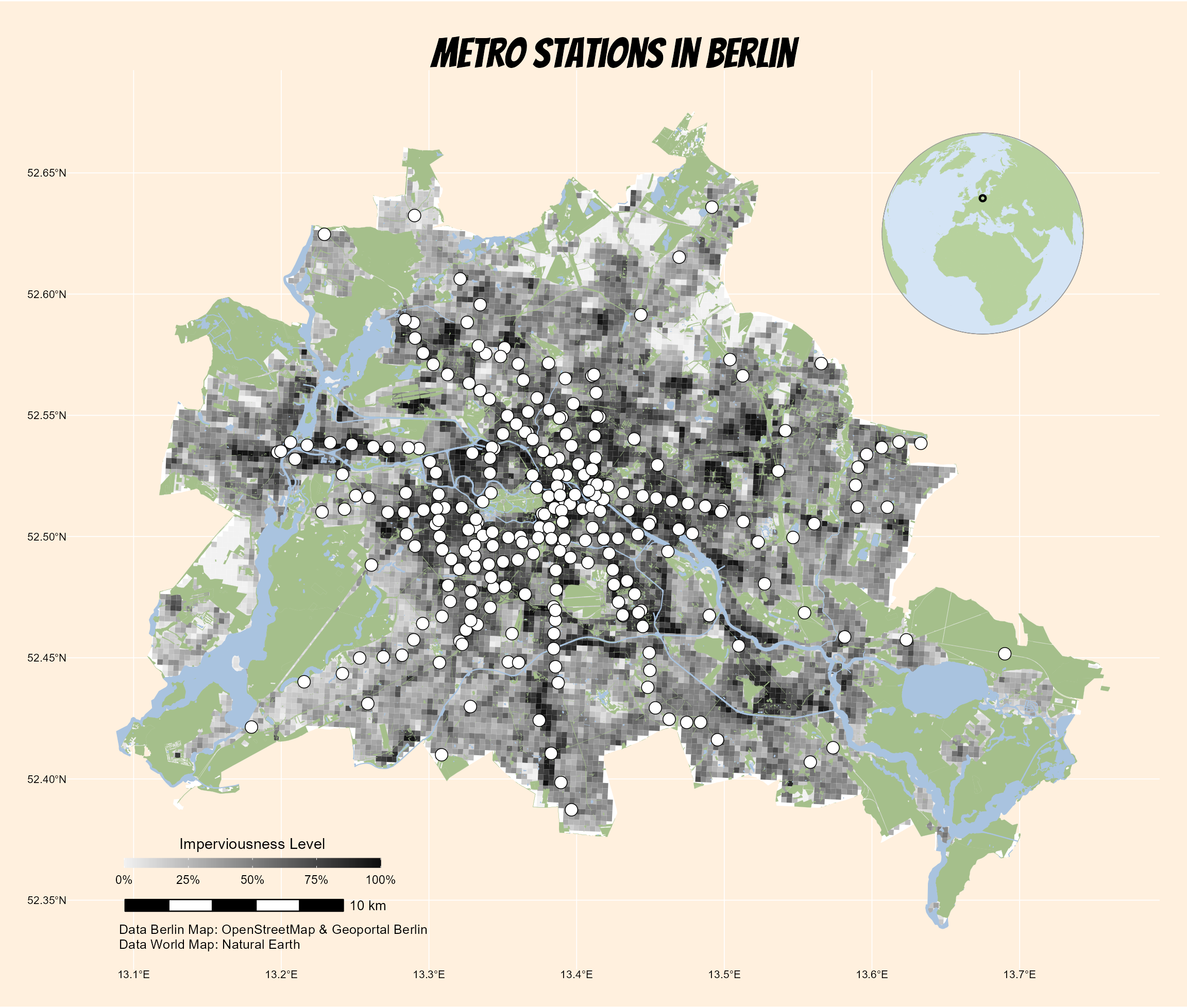

Save Map

Unfortunately, the size of the text elements is fixed. The best aspect ratio to export the map is 12x9 and you can save it with ggsave() for example:

ggsave("metro_map.pdf", width = 12, height = 9, device = cairo_pdf)

Spatial Datasets and Template Maps for Berlin