Clipping a Raster to a Specific Area

Learn how to use a clipping mask to extract a portion of a raster, based on a template extent. In this example we show you how to clip a raster map to the extent and borders of Berlin boundaries.

Sometimes you will get a dataset that is larger than your study area and you want to clip it to your specific extent or boundaries. There are two ways to do that:

• the crop function of the {terra} package: this will crop the dataset to the extent of the cropping mask
• the mask function of the {terra} package: this will crop the dataset to the extent of the cropping mask and set everything outside of the mask boundaries to NA (or to a custom set value)

In this tutorial only the mask function is covered because the crop function is straightforward to use. The mask function gives the opportunity to only get the raster cells that are covered by another raster or spatial object.

Here are two examples showing how to use data from the PopDynCloud and one with data from the geoboundaries website/package:

library(d6geodata)
library(sf)
library(terra)
library(dplyr)

Example PopDynCloud

If you have access to the PopDynCloud you can use the districts_berlin_layer like this:

berlin_mask <- get_geodata(data_name =  "districs_berlin_2022_poly_03035_gpkg",
                           path_to_cloud = "E:/PopDynCloud") # get_geodata function from the d6geodata package

Reading layer `districs_berlin_2022_poly_03035' from data source 
  `E:\PopDynCloud\GeoData\data-raw\berlin\districs_berlin_2022_poly_03035_gpkg\districs_berlin_2022_poly_03035.gpkg' 
  using driver `GPKG'
Simple feature collection with 97 features and 6 fields
Geometry type: MULTIPOLYGON
Dimension:     XY
Bounding box:  xmin: 4531043 ymin: 3253864 xmax: 4576654 ymax: 3290795
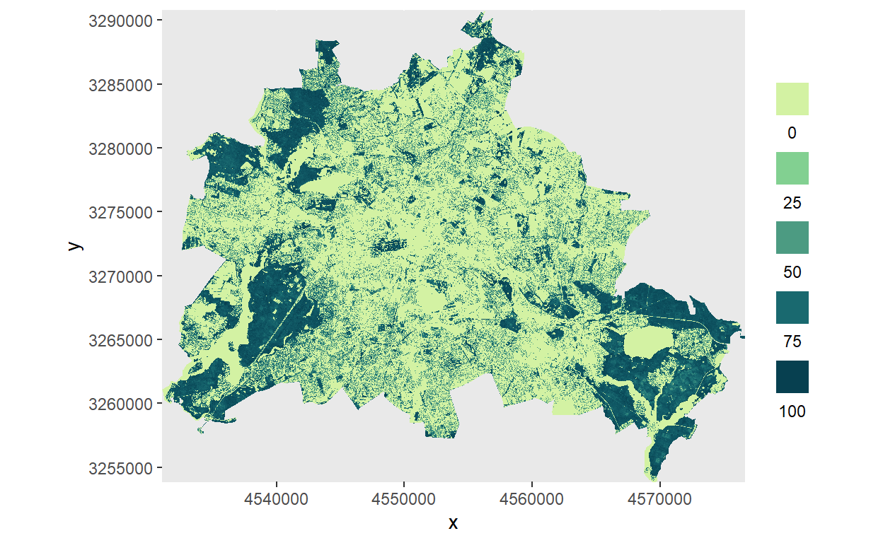
Projected CRS: ETRS89-extended / LAEA Europe

rast_example <- get_geodata(data_name =  "tree-cover-density_berlin_2018_10m_03035_tif",
                           path_to_cloud = "E:/PopDynCloud")


plot_quantitative_map(tif = rast_example) # plot not masked layer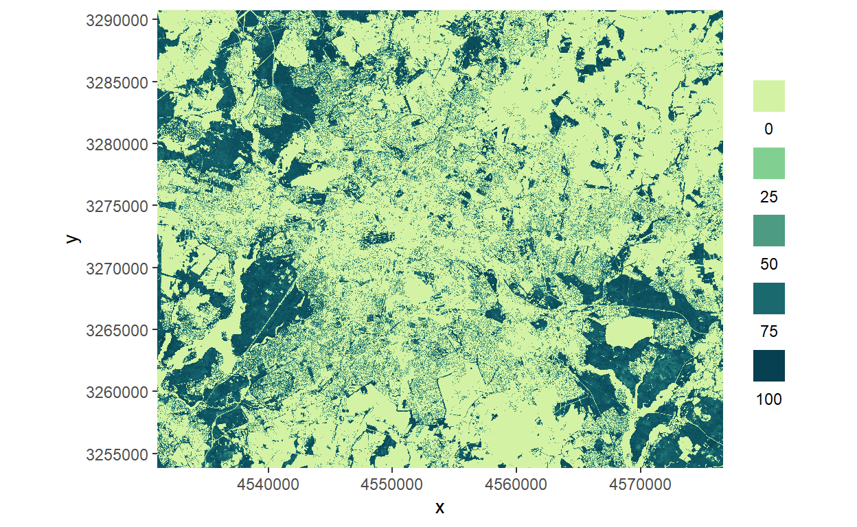

rast_example_masked <- mask(rast_example, # input raster 
                            berlin_mask) # mask to be clipped on 

plot_quantitative_map(tif = rast_example_masked) # plot masked layer

Example geoboundaries

If not, you can use the data from the geoboundaries website or using the rgeoboundaries package from github:

remotes::install_github("dickoa/rgeoboundaries")

library(rgeoboundaries)
rgeob_mask_berlin <- rgeoboundaries::gb_adm2("Germany") %>% # set Country name(s)
  filter(shapeName %in% "Berlin") %>% # filter for Berlin
  st_transform(3035) # reproject to 3035 (or desired crs) 

rast_example_rgeob_masked <- mask(rast_example, # input raster 
                                  rgeob_mask_berlin) # mask to be clipped on

plot_quantitative_map(tif = rast_example_rgeob_masked) # plot with function from d6geodata package