The NLRX package provides tools to setup and execute NetLogo simulations from R developed by Salecker et al. 2019. NetLogo is a free, open-source and cross-platform modelling environment for simulating natural and social phenomena.
Libraries and Folders
# libraries

for (pckg in c('dplyr', 'ggplot2', 'scico', 'nlrx'))
{
  if (!require(pckg, character.only = TRUE))
    install.packages(pckg, dependencies = TRUE)
  require(pckg, character.only = TRUE)
}

# output folder

currentDate <- gsub("-", "", Sys.Date())
# todaysFolder <- paste("Output", currentDate, sep = "_")
# dir.create(todaysFolder) #in case output folder is wanted

#virtual-ram if needed
#memory.limit(85000)
Setting Up the Library to Work with Your NetLogo Model
#NetLogo path
netlogoPath <- file.path("C:/Program Files/NetLogo 6.2.2/")

#Model location
modelPath <- file.path("./Model/myModel.nlogo")

#Output location (hardly ever used)
outPath <- file.path("./")

#Java
Sys.setenv(JAVA_HOME="C:/Program Files/Java/jre1.8.0_331")
Configure the NetLogo object:
nl <- nlrx::nl(
  nlversion = "6.2.2",
  nlpath = netlogoPath,
  modelpath = modelPath,
  jvmmem = 1024 # Java virtual machine memory capacity
)
Creating an Experiment
nl@experiment <- nlrx::experiment(
  expname = 'Exp_1_1',
  # name
  outpath = outPath,
  # outpath
  repetition = 1,
  # number of times the experiment is repeated with the !!!SAME!!! random seed
  tickmetrics = 'true',
  # record metrics at every step
  idsetup = 'setup',
  # in-code setup function
  idgo = 'go',
  # in-code go function
  runtime = 200,
  # soft runtime-cap
  metrics = c('population',  # global variables to be recorded, can also use NetLogos 'count' e.g. count turtles
              'susceptible', # but requires escaped quotation marks for longer commands when strings are involved
              'infected',    # functions similar for both patch and turtle variables (below)
              'immune'),
  metrics.patches = c('totalINfectionsHere',
                      'pxcor',
                      'pycor'),
 # metrics.turtles = list(
 #   "turtles" = c("xcor", "ycor")
 # ),
  constants = list(  # model parameters that are fixed. In theory all the constant values set in the UI before saving are the ones used
    'duration' = 20, # however, I would always make sure to 'fix" them though the constant input
    'turtle-shape' = "\"circle\"",
    'runtime' = 5
  ),
  variables = list( # model parameters you want to 'test' have several ways to be set
    'number-people' = list(values = c(150)),     # simple list of values
    'infectiousness' = list(                      #stepwise value change
      min = 50,
      max = 100,
      step = 25,
      qfun = 'qunif'
    ),
    # string based inputs such as used in NetLogo's 'choosers' or inputs require escaped quotation marks
    # "turtle-shape" = list(values = c("\"circle\"","\"person\"")),
    'chance-recover' = list(values = c(50, 75, 95))
  )
)
Creating a Simulation
Here we have several choices of simulation types. The full factorial simdesign used below creates a full-factorial parameter matrix with all possible combinations of parameter values. There are however, other options to choose from if needed and the vignette provides a good initial overview.
A bit counter intuitive but nseeds used in the simdesign is actually the number of repeats we want to use for our simulation. In case we set nseed = 10 and have set the the repetitions above to 1, we would run each parameter combination with 10 different random seeds i.e. 10 times per combination. If we would have set the repetitions to 2 we would run each random seed 2 times i.e. 20 times in total but twice for each seed so 2 results should be identical.
However, if your model handles seeds internally such as setting a random seed every time the model is setup, repetitions could be used instead.
nl@simdesign <- nlrx::simdesign_ff(nl=nl, nseeds=1)

print(nl)

nlrx::eval_variables_constants(nl)
Running the Experiment
Since the simulations are executed in a nested loop where the outer loop iterates over the random seeds of the simdesign, and the inner loop iterates over the rows of the parameter matrix. These loops can be executed in parallel by setting up an appropriate plan from the future package which is built into nlrx.
#plan(multisession, workers = 12) # one worker represents one CPU thread

results<- nlrx::run_nl_all(nl = nl)
to speed up this this tutorial we load a pre-generated simulation result
Rows: 1,809
Columns: 15
$ `[run number]`   <dbl> 1, 1, 1, 1, 1, 1, 1, 1, 1, 1, 1, 1, 1, 1, 1…
$ `number-people`  <dbl> 150, 150, 150, 150, 150, 150, 150, 150, 150…
$ infectiousness   <dbl> 50, 50, 50, 50, 50, 50, 50, 50, 50, 50, 50,…
$ `chance-recover` <dbl> 50, 50, 50, 50, 50, 50, 50, 50, 50, 50, 50,…
$ duration         <dbl> 20, 20, 20, 20, 20, 20, 20, 20, 20, 20, 20,…
$ `turtle-shape`   <chr> "circle", "circle", "circle", "circle", "ci…
$ runtime          <dbl> 5, 5, 5, 5, 5, 5, 5, 5, 5, 5, 5, 5, 5, 5, 5…
$ `random-seed`    <dbl> -662923684, -662923684, -662923684, -662923…
$ `[step]`         <dbl> 0, 1, 2, 3, 4, 5, 6, 7, 8, 9, 10, 11, 12, 1…
$ population       <dbl> 0, 153, 155, 156, 156, 157, 158, 159, 160, …
$ susceptible      <dbl> 0, 10, 10, 10, 11, 11, 13, 13, 16, 16, 17, …
$ infected         <dbl> 0, 143, 145, 146, 145, 146, 145, 146, 144, …
$ immune           <dbl> 0, 0, 0, 0, 0, 0, 0, 0, 0, 0, 0, 0, 0, 0, 0…
$ metrics.patches  <list> [<tbl_df[1225 x 5]>], [<tbl_df[1225 x 5]>]…
$ siminputrow      <dbl> 1, 1, 1, 1, 1, 1, 1, 1, 1, 1, 1, 1, 1, 1, 1…
NLRX output handling
There are several ways to use / analyze the output directly via nlrx (although I have not used them personally) detailed information can be found here: https://cran.r-project.org/web/packages/nlrx/nlrx.pdf
nlrx::setsim(nl, "simoutput") <- results # attaching simpout to our NetLogo object

#write_simoutput(nl) # having nlrx write the output into a file only works without patch or turtle metrics

nlrx::analyze_nl(nl, metrics = nlrx::getexp(nl, "metrics"), funs = list(mean = mean))
Cleaning the data
NetLogo really dislikes outputting nice and readable variable names so some renaming is in order:
raw1 <- results

raw2 <-
  raw1 %>% dplyr::rename(
    run = `[run number]`,
    recoveryChance = `chance-recover`,
    StartingPop = `number-people`,
    t = `[step]`
  )
In case of very large datasets we want to separate the patch (or turtle) specific data from the global data to speed up the analysis of the global data
globalData <- raw2 %>% dplyr::select(!metrics.patches)#, !metrics.turtles)and summarise like any other dataset
sum_1 <-
  globalData %>%
  dplyr::group_by(t, recoveryChance, infectiousness) %>%
  dplyr::summarise(
    across(
      c('infected',
        'immune',
        'susceptible',
        'population'),
      mean
    )
  ) %>%
  dplyr::filter(t < 201) %>%
  tidyr::pivot_longer(cols = -c(recoveryChance, infectiousness, t),
                      names_to = "EpiStat") %>%
  dplyr::ungroup()
Example plots
We use the global data to get an overview of the simulated SIR dynamics:
ggplot(sum_1) +
  geom_line(aes(x = t, y = value, colour = EpiStat), size = 1) +
  facet_grid(infectiousness ~ recoveryChance, labeller = label_both) +
  scale_colour_scico_d(
    palette = "lajolla",
    begin = 0.1,
    end = 0.9,
    direction = 1
  ) +
  theme_bw()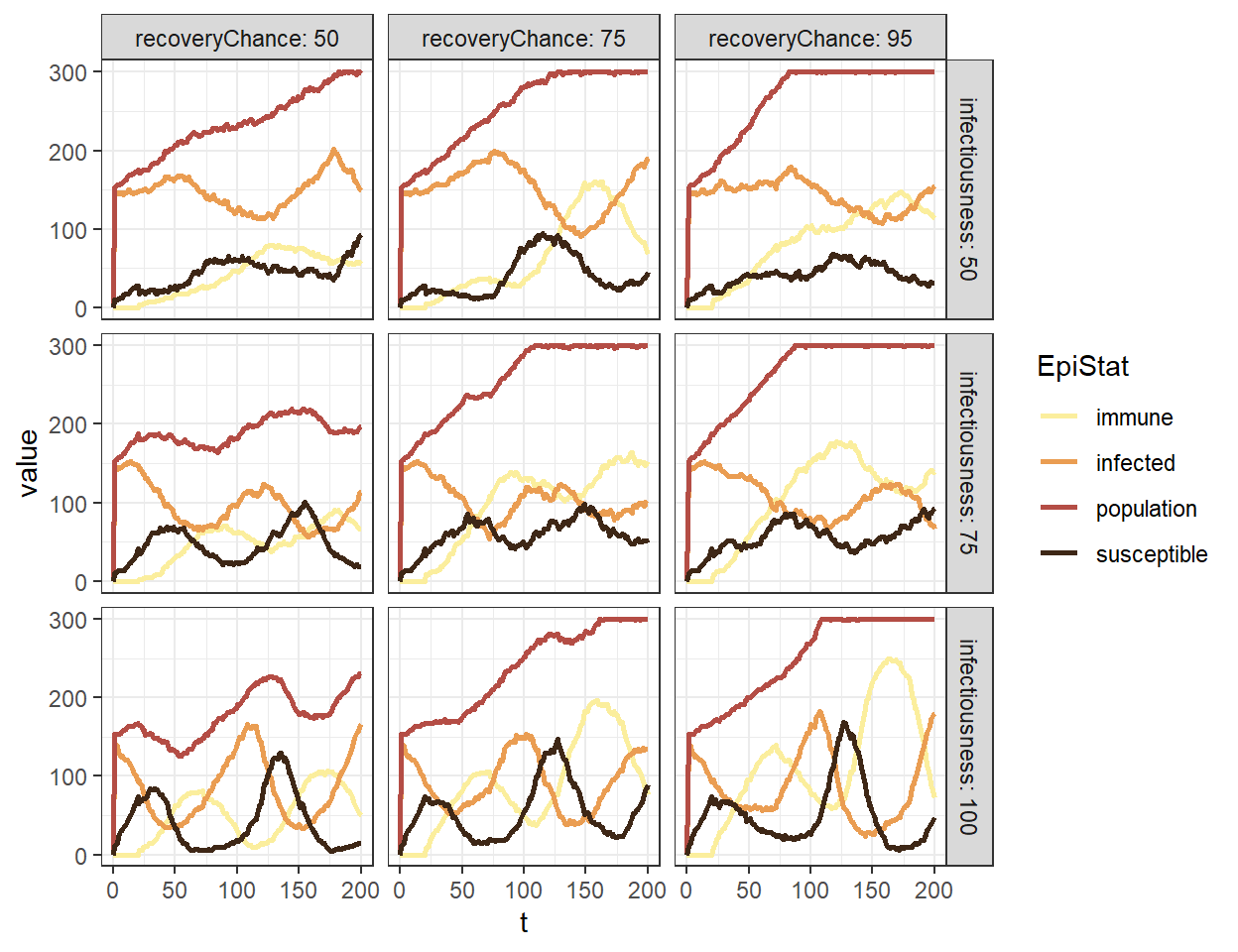
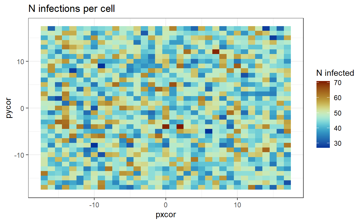
… and use the patch specific data to create a heatmap to visualize where most infections have happened in one specific scenario:
hmpRaw <- raw2 %>%
  dplyr::filter(infectiousness == 75 & recoveryChance == 75) %>%
  dplyr::select(metrics.patches, t) %>%
  dplyr::rename(pm = metrics.patches)

hmpSplit <- hmpRaw %>% split(hmpRaw$t)
tempDf <- hmpSplit[[1]]$pm
tempDf <- tempDf %>% as.data.frame() %>%
  dplyr::select(totalINfectionsHere, pxcor, pycor)

for (i in 1:length(hmpSplit))
{
  tmp1 <- as.data.frame(hmpSplit[[i]]$pm)
  colnames(tmp1) <- c(paste0("tab_", i), 'pxcor', 'pycor', 'agent', 'breed')
  tmp1 <- tmp1 %>%
    dplyr::select(-c('pxcor', 'pycor', 'agent', 'breed'))
  tempDf <- cbind(tempDf, tmp1)
}

tempDf2 <- tempDf %>%
  dplyr::select(-c(pxcor, pycor))

tempDf$summ <- rowSums(tempDf2)
hmpData <- tempDf %>% dplyr::select(summ, pxcor, pycor)

ggplot(hmpData)+
  geom_tile(aes(x = pxcor, y = pycor, fill = summ)) +
  scale_fill_scico(palette = 'roma', direction = -1, name= 'N infected') +
  ggtitle("N infections per cell") +
  theme_bw()